Chapter 13: Coupled Laws of Classical and Modern Engineering
In the winter of 1883 at Owens College in Manchester, engineering professor Osborne Reynolds stood beside an elevated glass-sided water tank six feet long to investigate how competing physical forces interact inside a moving fluid (Horowitz & Hill, 2015; Macaulay, 2016). Submerging a horizontal glass pipe with a polished wooden bell-mouth trumpet intake inside the tank, he allowed the water to stand undisturbed for hours until every stray thermal convection current had died away, and positioned a fine brass capillary tip connected to a reservoir of dark carmine dye just upstream of the intake. When Reynolds cracked open the discharge valve slightly so water crept through the glass pipe at a gentle velocity \(v\), the streak of crimson dye drawn into the intake formed a razor-sharp, steady thread down the exact centerline of the tube—so still that it looked like a solid rod of ruby glass suspended in clear crystal as concentric layers (laminae) of water slid past one another without a trace of radial mixing.
As Reynolds slowly opened the valve further, the velocity \(v\) climbed until, at a sharply defined threshold, a hydrodynamic instability seized the stream: several feet downstream of the intake, the crimson filament suddenly began to waver, curled into a train of interlocking vortices, and burst into a cloud of chaotic three-dimensional eddies that tinted the entire bore of the pipe pink. When he illuminated the tube with a microsecond electric spark, the uniform pink blur resolved into tightly wound, tumbling vortices. By repeating the experiment across glass pipes of different diameters \(D\) and heating the water to vary its dynamic viscosity \(\mu\) and density \(\rho\), Reynolds proved that the transition from tranquil laminae to chaotic eddies depends on a single dimensionless ratio \(\text{Re} = \rho v D / \mu\)—where fluid inertia competes against viscous shear—rather than on velocity, pipe size, or viscosity in isolation (Horowitz & Hill, 2015; Macaulay, 2016).
Across classical and modern engineering, no physical system obeys a single isolated formula: viscous shear competes with fluid inertia, thermal conduction feeds convective and radiative dissipation, optical diffraction couples with lens curvature, and orbital gravity balances rocket mass expulsion. Evaluating these coupled systems from their innermost dimensionless ratio outward keeps each intermediate state—Reynolds number \(\text{Re}\), hydraulic radius \(R_h\), Euler buckling load \(P_{\text{cr}}\), log-mean temperature difference \(\Delta T_{\text{lm}}\), numerical aperture \(\text{NA}\), objective magnification \(m_o\), or circular orbital velocity \(v_{\text{orb}}\)—visible on the stack at the boundary where one physical mechanism hands off to the next (Figure 13.1).
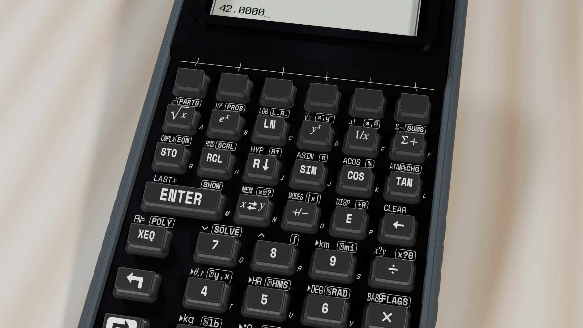
13.1 Viscous Pipe Flow, Open-Channel Hydraulics & Heat Transfer
Why does blood plasma glide silently through a microscopic capillary without mixing, while water rushing through a municipal fire main churns in violent eddies? For two centuries of early hydrodynamics, frictionless differential models predicted zero drag on a moving submarine (d'Alembert's paradox), while practical hydraulic tables for cast-iron pipes and earthen canals seemed disconnected from first principles.
13.1.1 The Reynolds Regime Boundary, Hagen–Poiseuille Capillaries & Stokes Drag
Reynolds's 1883 pipe experiments resolved that divide by comparing a moving fluid's density \(\rho\), mean cross-sectional velocity \(v\), and conduit diameter \(D\) against its dynamic viscosity \(\mu\) (or kinematic viscosity \(\nu = \mu/\rho\)), collapsing the ratio of convective momentum flux (\(\rho v^2 / D\)) to viscous shear stress (\(\mu v / D^2\)) into a single dimensionless number:
Fluid density \(\rho\), speed \(v\), and pipe bore \(D\) combine in \(\rho v D\) to drive the stream's forward momentum and vortex formation, while dynamic viscosity \(\mu\) acts as internal molecular friction that damps lateral disturbances back into parallel laminae. Across all Newtonian liquids and gases in circular conduits, viscous shear preserves smooth laminar flow for \(\text{Re} < 2,300\); intermittent turbulent slugs appear across the transitional band \(2,300 \le \text{Re} \le 4,000\); and inertial eddies dominate in fully turbulent flow for \(\text{Re} > 4,000\).
In the laminar regime (\(\text{Re} < 2,300\)), viscous flow in a circular capillary tube of radius \(r = D/2\) and length \(L\) under pressure differential \(\Delta P\) departs sharply from uniform plug flow. Fluid molecules touching the stationary pipe wall are held at zero velocity (\(u(r) = 0\), the no-slip boundary condition), while nested cylindrical shells of fluid closer to the axis telescope forward under the axial pressure force \(\pi r'^2 \Delta P\), resisted by viscous shear stress \(\tau = -\mu\frac{du}{dr'}\) around their circumference \(2\pi r' L\). Integrating this force balance yields a parabolic velocity distribution \(u(r') = \frac{\Delta P}{4\mu L}(r^2 - r'^2)\) whose centerline speed is twice the mean velocity, and integrating that paraboloid across the circular cross-section yields the Hagen–Poiseuille Law for volumetric flow rate \(Q\):
While pressure drop \(\Delta P\) drives the discharge and viscosity \(\mu\) and tube length \(L\) throttle it back, volumetric flow \(Q\) scales with the fourth power of radius (\(r^4\)) because two quadratic effects reinforce each other: doubling the tube radius \(r\) quadruples the cross-sectional area \(\pi r^2\), and moving the core stream twice as far from the stationary walls quadruples the centerline speed of the parabolic velocity profile (\(2^2 \times 2^2 = 2^4 = 16\)).
This \(r^4\) sensitivity governs flow resistance across physiology, chemical instrumentation, and microfluidics. In coronary and vascular perfusion, if atherosclerotic plaque narrows the internal radius of a coronary arteriole by just \(16\%\) (\(r' = 0.84\,r\)), the vessel's cross-sectional area drops by \(29\%\), but its laminar blood flow capacity at constant blood pressure plummets by half (\(0.84^4 \approx 0.498 \approx 50\%\)). When a tissue bed instead requires constant blood flow \(Q\) while vasoconstriction reduces arteriole radius by half (\(r' = 0.5\,r\)), the required driving pressure differential \(\Delta P \propto r^{-4}\) spikes sixteenfold.
When blood plasma (\(\rho = 1,025\text{ kg/m}^3,\; \mu = 1.5 \times 10^{-3}\text{ Pa}\cdot\text{s}\)) flows through a \(D = 4\text{ mm}\) vessel at \(v = 0.45\text{ m/s}\), the Reynolds number is \(\text{Re} = 1025(0.45)(0.004) / (1.5 \times 10^{-3}) = \mathbf{1,230}\)—well within the laminar regime (\(\text{Re} < 2,300\)). In a microfluidic fused-silica capillary of inner radius \(r = 250\,\mu\text{m}\) (\(2.5 \times 10^{-4}\text{ m}\)) and length \(L = 0.15\text{ m}\) carrying water (\(\mu \approx 1.002 \times 10^{-3}\text{ Pa}\cdot\text{s}\)) under pressure drop \(\Delta P = 45,000\text{ Pa}\), the fourth power of radius (\(r^4 \approx 3.906 \times 10^{-15}\text{ m}^4\)) scaled by \(\pi\Delta P / (8\mu L)\) yields a laminar discharge of \(Q \approx \mathbf{4.593 \times 10^{-7}\text{ m}^3/\text{s}}\) (\(\approx 0.459\text{ mL/s}\)).
For external flow around a small solid sphere of radius \(r\) and particle density \(\rho_p\) moving at slow velocity \(v\) through an unbounded viscous fluid of density \(\rho_f\) and dynamic viscosity \(\mu\) under standard gravity \(g_0\) (\(\text{Re} \ll 1\)), convective inertia is negligible compared to viscous shear and streamlines wrap symmetrically fore-and-aft around the sphere without separating into a wake. Integrating the surface pressure and viscous shear tensor over the sphere yields Stokes's Law of Creeping Drag \(F_d\) and the Stokes Terminal Sedimentation Velocity \(v_t\) (where upward viscous drag \(6\pi\mu r v_t\) balances downward net buoyant weight \(\frac{4}{3}\pi r^3(\rho_p - \rho_f)g_0\)):
Creeping viscous drag \(F_d\) grows only linearly with viscosity \(\mu\), sphere radius \(r\), and speed \(v\). As a particle settles under gravity, its downward buoyant weight scales with volume (\(\propto r^3(\rho_p - \rho_f)g_0\)) while opposing viscous drag scales only with radius (\(\propto \mu r\)), leaving a terminal settling speed \(v_t\) proportional to the square of particle radius (\(r^2\)) and inversely proportional to \(\mu\): a \(100\,\mu\text{m}\) fine sand grain settles through water one hundred times faster than a \(10\,\mu\text{m}\) silt particle, allowing civil water-treatment clarifiers and geological elutriators to sort grains by size. In a laboratory falling-ball viscometer, dropping a precision steel bearing of radius \(r = 1\text{ mm}\) (\(\rho_p = 7,850\text{ kg/m}^3\)) through pharmaceutical glycerin (\(\rho_f = 1,260\text{ kg/m}^3,\; \mu = 0.95\text{ Pa}\cdot\text{s}\)) under \(g_0 \approx 9.807\text{ m/s}^2\) produces a creeping terminal speed of \(v_t = \frac{2(10^{-3})^2(6,590)(9.807)}{9(0.95)} \approx \mathbf{0.015\text{ m/s}}\) (\(\approx 15.12\text{ mm/s}\), at \(\text{Re} \approx 0.04\)) and a Stokes viscous drag force of \(F_d \approx \mathbf{2.707 \times 10^{-4}\text{ N}}\).
13.1.2 Turbulent Darcy–Weisbach Mains, Open-Channel Hydraulics & Column Buckling
Above Reynolds's transition boundary lies the turbulent regime (\(\text{Re} > 4,000\)) of city water mains, hydroelectric penstocks, and transcontinental petroleum pipelines. Once \(\text{Re}\) exceeds \(4,000\), turbulent eddies continuously sweep high-velocity fluid from the pipe centerline out toward the walls and fling slow near-wall fluid back into the core. This radial momentum exchange flattens the laminar paraboloid into a blunt, nearly uniform velocity plug across \(95\%\) of the pipe bore, while concentrating an intense velocity gradient inside a paper-thin viscous sublayer clinging to the pipe wall.
Because momentum transport across the core is now driven by inertial eddies of kinetic energy density \(\frac{1}{2}\rho v^2\) rather than molecular viscosity \(\mu\), frictional head loss \(\Delta h_f\) (in meters of fluid column) over a pipe of length \(L\), internal diameter \(D\), internal wall roughness height \(\varepsilon\), and volumetric flow rate \(Q = \frac{\pi}{4}D^2 v\) is proportional to the dimensionless Darcy friction factor \(f\) and the square of mean velocity under the Darcy–Weisbach and Colebrook–White Equations (Colebrook, 1939):
The two forms of the Darcy–Weisbach equation show how pipe geometry governs head loss: the first form multiplies the friction factor \(f\) by the length-to-diameter aspect ratio \(L/D\) and the velocity head \(\frac{v^2}{2g_0}\). Substituting \(v = \frac{4Q}{\pi D^2}\) for a fixed volumetric discharge \(Q\) makes velocity head scale as \(v^2 \propto Q^2 / D^4\), which multiplied by \(L/D\) reveals that turbulent frictional head loss scales inversely with the fifth power of pipe diameter (\(\Delta h_f \propto Q^2 / D^5\)). Halving the diameter of a municipal water main from \(400\text{ mm}\) to \(200\text{ mm}\) to save cast-iron pipe cost multiplies the frictional pumping head loss thirty-two-fold (\(2^5 = 32\)).
Two boundary-layer mechanisms compete inside Colebrook and White's logarithmic argument: the geometric relative roughness term \(\frac{\varepsilon / D}{3.7}\) and the viscous sublayer thickness term \(\frac{2.51}{\text{Re}\sqrt{f}}\). At moderate Reynolds numbers, the viscous sublayer is thicker than the wall roughness elements \(\varepsilon\), so the second term dominates, the pipe behaves as hydraulically smooth, and \(f\) falls as \(\text{Re}\) increases. At high Reynolds numbers, the viscous sublayer thins until the roughness peaks \(\varepsilon\) pierce right through it, shedding form-drag vortices; in this fully rough zone, the \(2.51/(\text{Re}\sqrt{f})\) term vanishes and \(f\) depends solely on the relative roughness \(\varepsilon/D\). For a municipal steel water main of length \(L = 450\text{ m}\) and internal diameter \(D = 0.2\text{ m}\) (\(L/D = 2,250\)) carrying water at \(v = 2.4\text{ m/s}\) with Moody friction factor \(f = 1.85 \times 10^{-2}\) under \(g_0 \approx 9.807\text{ m/s}^2\), the Darcy–Weisbach head loss is \(\Delta h_f = 1.85 \times 10^{-2}(2,250)(2.4^2)/(2 \times 9.807) \approx \mathbf{12.224\text{ m}}\) (\(\approx 119.88\text{ kPa}\)).
Whereas viscous wall friction dissipates mechanical energy irreversibly over long pipe runs (\(L/D \gg 1\)), accelerating a fluid of density \(\rho\) and upstream speed \(v_1\) through a short, smooth pipe constriction from upstream diameter \(D_1\) to throat diameter \(D_2\) reversibly trades static pressure \(P\) for dynamic pressure \(\frac{1}{2}\rho v^2\) in a Venturi Meter (\(\Delta P_{\text{Venturi}} = P_1 - P_2\)). When the flowing medium is a compressible gas at absolute temperature \(T\) with adiabatic heat-capacity ratio \(\gamma = c_p / c_v\) and specific gas constant \(R_{\text{air}}\), pressure disturbances propagate at the adiabatic speed of sound \(a\), and the ratio of flow speed \(v\) to \(a\) defines the dimensionless Mach number \(M\):
Mass continuity \(A_1 v_1 = A_2 v_2\) forces the throat velocity in a Venturi constriction to climb with the square of the diameter ratio as \(v_2 = v_1(D_1/D_2)^2\), so squaring velocity in Bernoulli's dynamic pressure \(\frac{1}{2}\rho(v_2^2 - v_1^2)\) makes the static pressure drop scale with the fourth power of the diameter ratio \((D_1/D_2)^4 - 1\). Acoustic speed \(a = \sqrt{\gamma R_{\text{air}} T}\) meanwhile depends only on the square root of absolute temperature \(T\) (and not on ambient pressure) because sound waves are microscopic pressure pulses relayed from molecule to molecule by thermal collisions, whose mean molecular speed scales as \(\sqrt{T}\). When water (\(\rho = 1,000\text{ kg/m}^3\)) flowing at upstream speed \(v_1 = 2\text{ m/s}\) enters a Venturi meter that narrows from \(D_1 = 0.15\text{ m}\) to throat \(D_2 = 0.075\text{ m}\) (\(D_1/D_2 = 2\)), the fourth-power factor \(2^4 - 1 = 15\) multiplied by upstream dynamic pressure \(\frac{1}{2}(1,000)(2^2) = 2,000\text{ Pa}\) produces a static pressure drop of \(\Delta P_{\text{Venturi}} = \mathbf{30,000\text{ Pa}}\) (\(30\text{ kPa}\)). At stratospheric cruise altitude (\(11,000\text{ m},\; T = 216.65\text{ K}\)) with \(\gamma = 1.4\) and \(R_{\text{air}} \approx 287.058\text{ J/(kg}\cdot\text{K)}\), local sonic speed is \(a \approx \mathbf{295.07\text{ m/s}}\), so an airliner cruising at true airspeed \(v = 250.8\text{ m/s}\) operates at Mach number \(M = 250.8 / 295.07 \approx \mathbf{0.85}\).
If the top of a pressurized pipe is opened to the atmosphere—as in a hydroelectric tailrace flume, a concrete storm-drainage floodway, or a mountain river—atmospheric pressure acts equally on the free surface at every station along the channel, leaving no hydrostatic pressure gradient \(\Delta P / L\) to drive the flow. Steady uniform flow is driven instead by the downslope component of gravity, represented by the longitudinal bed slope \(S = \sin\theta \approx \Delta z / L\), which is balanced by turbulent boundary shear along the solid channel floor and walls characterized by Manning's empirical surface roughness coefficient \(n\) (\(n = 0.013\) for troweled concrete, \(0.025\) for natural earth canals, and \(0.04\) for cobble-bed mountain streams).
The governing geometric scale of any open channel is its Hydraulic Radius \(R_h\)—defined as the ratio of the wetted cross-sectional flow area \(A\) to the solid wetted perimeter \(P_{\text{wet}}\) in contact with the water (excluding the free air interface)—which determines mean channel velocity \(v\) and volumetric discharge \(Q\) in Manning's Equation:
Because the hydraulic radius \(R_h = A / P_{\text{wet}}\) compares the water cross-section \(A\) pulled downhill by gravity against the solid perimeter \(P_{\text{wet}}\) retarding it by wall shear, raising \(R_h\) to the \(2/3\) power rewards deep, compact channels, the square root of bed slope \(S^{1/2}\) reflects quadratic turbulent drag (\(S \propto v^2\)), and dividing by \(n\) penalizes rough channel beds. For a full circular pipe of diameter \(D\), \(R_h = (\pi D^2/4)/(\pi D) = D/4\)—and the same \(R_h = D/4\) holds for a half-full semicircular channel, since both area and wetted perimeter are halved.
If a civil engineer excavates a cross-sectional area of \(A = 6\text{ m}^2\) as a wide, shallow tray (\(w = 12\text{ m}\) wide by \(d = 0.5\text{ m}\) deep), the wetted perimeter \(P_{\text{wet}} = w + 2d = 13\text{ m}\) drags heavily on the flow (\(R_h = 6/13 \approx 0.462\text{ m}\)). Proportioning that same \(A = 6\text{ m}^2\) as a compact rectangular concrete channel of width \(w = 4\text{ m}\) and depth \(d = 1.5\text{ m}\) (where \(d = w/2\) is the optimal rectangular proportion minimizing \(P_{\text{wet}}\) for a given area) cuts the wetted perimeter to \(P_{\text{wet}} = 4 + 2(1.5) = 7\text{ m}\), nearly doubles the hydraulic radius to \(R_h = 6/7 \approx 0.857\text{ m}\), and at slope \(S = 1.6 \times 10^{-3}\) with \(n = 0.013\) conveys \(Q \approx \mathbf{16.659\text{ m}^3/\text{s}}\) at mean speed \(v \approx \mathbf{2.776\text{ m/s}}\).
Where Reynolds showed that a laminar stream loses stability and breaks into turbulent eddies above a critical threshold, Leonhard Euler showed that a slender structural column of length \(L\), cross-sectional area \(A\), Young's modulus \(E\), and weak-axis area moment of inertia \(I\) (with radius of gyration \(r_g = \sqrt{I/A}\)) under axial compression does not fail by crushing at the material's yield stress \(\sigma_y\). Instead, at the Euler critical buckling load \(P_{\text{cr}}\)—governed by its flexural stiffness \(EI\) and its effective buckling length \(KL\) (or dimensionless slenderness ratio \(\lambda = KL/r_g\)), where \(K\) is the effective length factor set by the rotational and translational restraints at the column ends—the straight column suddenly bows sideways into a sinusoidal buckle:
Flexural rigidity \(\pi^2 E I\) resists lateral bowing into a half-sine wave while the effective unbraced length \((KL)^2\) reduces stability quadratically—or equivalently, axial stiffness \(\pi^2 E A\) is divided by the square of the dimensionless slenderness ratio \((KL/r_g)^2\):
| End Support Boundary Condition | Theoretical \(K\) | Design \(K\) (AISC) | Effective Buckling Wavelength \(L_{\text{eff}} = K L\) | Relative Buckling Capacity \(P_{\text{cr}} / P_{\text{pinned}}\) |
|---|---|---|---|---|
| Pinned–Pinned (Both ends free to rotate, fixed against translation) | \(1\) | \(1\) | \(1\,L\) (Fundamental half-sine wave) | \(1\times\) |
| Fixed–Fixed (Both ends built-in against rotation and translation) | \(0.5\) | \(0.65\) | \(0.5\,L\) (Inflection points at \(L/4\) and \(3L/4\)) | \(4\times\) |
| Fixed–Pinned (Base fixed, top pinned against lateral sway) | \(0.699\) (\(\approx 0.7\)) | \(0.8\) | \(0.7\,L\) (\(\tan(\pi/K) = \pi/K\) root) | \(2.04\times\) |
| Fixed–Free (Flagpole cantilever: base fixed, top free to sway) | \(2\) | \(2.1\) | \(2\,L\) (Quarter-sine wave; mirrors virtual \(2L\) column) | \(0.25\times\) |
Because \(P_{\text{cr}}\) scales as \(K^{-2}\), welding both ends of a pinned column rigid against rotation (\(K = 0.5\)) moves the inflection points inward to the quarter-span points and quadruples its elastic buckling capacity (\(4\times\)); freeing the top of a column to sway laterally like a flagpole (\(K = 2\)) cuts its buckling capacity to one-quarter (\(0.25\times\)). For a pinned-end (\(K = 1\)) structural steel column of length \(L = 3\text{ m}\), Young's modulus \(E = 200\text{ GPa}\), and weak-axis moment of inertia \(I = 8 \times 10^{-6}\text{ m}^4\) (\(800\text{ cm}^4\)), the flexural rigidity product \(\pi^2 E I \approx 1.579 \times 10^7\text{ N}\cdot\text{m}^2\) divided by \((KL)^2 = 9\text{ m}^2\) yields a critical buckling load of \(P_{\text{cr}} \approx \mathbf{1,754,596.34\text{ N}}\) (\(\approx 1.755\text{ MN}\)).
Across horizontal bridge spans and rotating machinery drive trains, two companion elasticity laws govern serviceability and stress. First, a pin-supported steel bridge girder (\(E = 200\text{ GPa}\), strong-axis \(I = 1.25 \times 10^{-4}\text{ m}^4\)) spanning \(L = 8\text{ m}\) (\(L^4 = 4,096\text{ m}^4\)) under a uniform floor load \(w = 18,000\text{ N/m}\) experiences a mid-span deflection of \(\delta_{\max} = \frac{5 w L^4}{384 E I} = 3.84 \times 10^{-2}\text{ m}\) (\(\mathbf{38.4\text{ mm}}\)). Second, a solid circular marine propeller shaft of diameter \(d = 0.12\text{ m}\) and length \(L = 4.5\text{ m}\) machined from Monel alloy (shear modulus \(G = 65\text{ GPa}\)) transmitting continuous torque \(T = 24,000\text{ N}\cdot\text{m}\) experiences peak outer-fiber shear stress \(\tau_{\max} = \frac{16 T}{\pi d^3} \approx \mathbf{70.736\text{ MPa}}\), while scaling \(\tau_{\max}\) by \(\frac{2L}{Gd}\) gives an end-to-end torsional twist angle of \(\theta = \frac{32 T L}{\pi G d^4} \approx \mathbf{0.082\text{ rad}}\) (\(\approx \mathbf{4.676^\circ}\)).
13.1.3 Heat Engines, Counter-Flow Exchangers, Room Acoustics & RF Links
The Second Law of Thermodynamics sets a hard upper bound on the thermal efficiency of any heat engine, regardless of working fluid. Because heat cannot perform mechanical work by itself, work is extracted only when thermal energy falls across a temperature difference from a hot source at absolute temperature \(T_H\) to a cold sink at \(T_C\) (in Kelvin, \(T_{\text{K}} = T_{^\circ\text{C}} + 273.15\)), bounded for any reversible cycle by the Carnot Efficiency:
Maximum work extraction is bounded by the fraction of absolute thermal energy that drops between \(T_H\) and \(T_C\), while the remaining share \(T_C / T_H\) is the unavoidable fraction of input heat that must be rejected to the cold sink to export entropy. In a combined-cycle power plant receiving heat at \(T_H = 850\text{ K}\) (\(576.85^\circ\text{C}\)) and rejecting waste heat to a cooling tower at \(T_C = 300\text{ K}\) (\(26.85^\circ\text{C}\)), the Carnot limit is \(\eta_{\text{Carnot}} = 1 - 300/850 \approx \mathbf{0.647}\) (\(\approx 64.71\%\)).
To transfer thermal power \(q\) between process streams without mixing them, chemical plants and power stations use Counter-Flow Shell-and-Tube Heat Exchangers of overall heat-transfer conductance \(U\) (\(\text{W/(m}^2\cdot\text{K)}\)) and total tube surface area \(A\) (\(\text{m}^2\)) (Incropera et al., 2007). Because the local temperature difference \(\Delta T(x) = T_h(x) - T_c(x)\) decays exponentially along the exchanger length \(x\), integrating the local heat-transfer rate law \(dq = U\,\Delta T(x)\,dA\) from terminal temperature difference \(\Delta T_1 = T_{h,\text{in}} - T_{c,\text{out}}\) at End 1 to \(\Delta T_2 = T_{h,\text{out}} - T_{c,\text{in}}\) at End 2 yields the total heat-transfer rate \(q\) in terms of the Log-Mean Temperature Difference (\(\text{LMTD}\), \(\Delta T_{\text{lm}}\)):
Scaling the end-to-end difference \(\Delta T_1 - \Delta T_2\) by the logarithmic ratio \(\ln(\Delta T_1 / \Delta T_2)\) accounts for the exponential decay of the temperature gap along the tubes, yielding an effective driving temperature difference \(\Delta T_{\text{lm}}\) that always lies between the geometric mean \(\sqrt{\Delta T_1 \Delta T_2}\) and the arithmetic mean \(\frac{1}{2}(\Delta T_1 + \Delta T_2)\). For terminal differences \(\Delta T_1 = 65\text{ K}\) and \(\Delta T_2 = 25\text{ K}\), dividing \(65 - 25 = 40\text{ K}\) by \(\ln(65/25) = \ln(2.6) \approx 0.956\) gives \(\Delta T_{\text{lm}} \approx \mathbf{41.862\text{ K}}\)—more than \(3.1\text{ K}\) below the arithmetic mean of \(45\text{ K}\).
Alongside convective heat exchangers, three thermal and phase-equilibrium laws govern process and aerospace thermal engineering. First, the Clausius–Clapeyron Vapor-Pressure Equation relates saturation vapor pressure \(P_2\) at absolute temperature \(T_2\) to a reference boiling point \((P_1, T_1)\) via molar enthalpy of vaporization \(\Delta H_{\text{vap}}\) and universal gas constant \(R \approx 8.314\text{ J/(mol}\cdot\text{K)}\):
The ratio \(\Delta H_{\text{vap}} / R\) sets the characteristic vaporization temperature scale, and multiplying by the reciprocal temperature shift \(\left(\frac{1}{T_1} - \frac{1}{T_2}\right)\) tracks the Boltzmann fraction of liquid molecules energetic enough to break free into the vapor phase. For water (\(\Delta H_{\text{vap}} = 40,650\text{ J/mol},\; P_1 = 101.325\text{ kPa}\) at \(T_1 = 373.15\text{ K}\)) atop a \(3,000\text{ m}\) mountain pass where water boils at \(T_2 = 363.15\text{ K}\) (\(90^\circ\text{C}\)), the inverse temperature difference \(\frac{1}{373.15} - \frac{1}{363.15} \approx -7.381 \times 10^{-5}\text{ K}^{-1}\) scaled by \(\Delta H_{\text{vap}}/R\) and exponentiated gives an atmospheric boiling pressure of \(P_2 \approx \mathbf{70.636\text{ kPa}}\).
Second, by the Stefan–Boltzmann Law \(P_{\text{rad}} = \varepsilon\sigma A(T^4 - T_{\text{amb}}^4)\) with \(\sigma \approx 5.67 \times 10^{-8}\text{ W/(m}^2\cdot\text{K}^4)\) (Incropera et al., 2007), a spacecraft radiator panel of area \(A = 2.5\text{ m}^2\) and emissivity \(\varepsilon = 0.88\) at \(T = 320\text{ K}\) (\(320^4 \approx 1.049 \times 10^{10}\text{ K}^4\)) radiating into \(T_{\text{amb}} = 4\text{ K}\) deep space rejects \(P_{\text{rad}} \approx \mathbf{1,307.99\text{ W}}\). Third, when steady radial heat-loss rate \(q\) (\(\text{W}\)) flows from an inner steam pipe at temperature \(T_{\text{inner}}\) through a cylindrical mineral-wool insulation sleeve (inner radius \(r_1 = 0.05\text{ m}\), outer radius \(r_2 = 0.09\text{ m}\), length \(L = 10\text{ m}\), thermal conductivity \(k = 0.042\text{ W/(m}\cdot\text{K)}\)) and convects from the outer jacket into ambient plant air at temperature \(T_\infty\) with convective heat-transfer coefficient \(h_{\text{conv}} = 12\text{ W/(m}^2\cdot\text{K)}\), the cylindrical conduction resistance \(R_{\text{cond}}\) and outer convection resistance \(R_{\text{conv}}\) act in series (Incropera et al., 2007):
Cylindrical conduction resistance \(R_{\text{cond}}\) depends on the natural logarithm \(\ln(r_2 / r_1)\) rather than the linear wall thickness \((r_2 - r_1)\) because the heat-flow circumference \(2\pi r L\) widens in direct proportion to radius \(r\) as heat moves outward from \(r_1\) to \(r_2\), so integrating the local radial resistance \(dr / (2\pi r k L)\) across the shell produces \(\frac{\ln(r_2/r_1)}{2\pi k L}\). At the outer jacket \(r_2\), heat crosses the boundary layer of area \(2\pi r_2 L\) against convection resistance \(R_{\text{conv}} = \frac{1}{2\pi r_2 L h_{\text{conv}}}\); because the same thermal power \(q\) traverses the insulation and the surrounding air film in succession, \(R_{\text{cond}}\) and \(R_{\text{conv}}\) add in series just like electrical resistors in Ohm's law.
In architectural acoustics, a spoken syllable in an untreated stone or plaster hall echoes for several seconds because hard surfaces absorb only a small fraction of incident sound energy on each reflection. When an enclosure of volume \(V\) (\(\text{m}^3\)) is bounded by \(N\) surface panels of individual areas \(S_i\) (\(\text{m}^2\), summing to total room surface area \(S_{\text{tot}} = \sum_{i=1}^N S_i\)) and dimensionless sound absorption coefficients \(\alpha_i \in [0, 1]\), their weighted sum defines the total equivalent absorption area \(A_{\text{abs}} = \sum_{i=1}^N S_i \alpha_i\) (in metric sabins, \(\text{m}^2\)) and the area-weighted average absorption coefficient \(\bar{\alpha} = A_{\text{abs}} / S_{\text{tot}}\). The reverberation time \(RT_{60}\)—the time required for acoustic energy density in the room to decay by \(60\text{ dB}\) (one-millionth of its initial intensity)—is governed by Sabine's Reverberation Equation in live halls and by the Norris–Eyring Reverberation Equation (which models discrete mean-free-path wall reflections where each bounce multiplies surviving acoustic energy by \((1 - \bar{\alpha})\)) in heavily damped broadcast studios:
Room volume \(V\) drives the \(0.161\,V\) factor (where \(0.161\text{ s/m} = \frac{24\ln 10}{c}\) at room sound speed \(c \approx 343\text{ m/s}\)) because sound waves travel longer free paths between wall collisions in a larger hall, whereas the surface-absorption terms govern how rapidly each reflection drains acoustic energy. The Norris–Eyring logarithm \(-\ln(1 - \bar{\alpha})\) resolves the total-absorption limit: as wall absorption approaches perfection (\(\bar{\alpha} \to 1\)), \(-\ln(1 - \bar{\alpha}) \to \infty\) drives \(RT_{60,\text{Eyring}} \to 0\) as physically required, while for live concert halls (\(\bar{\alpha} \ll 1\)), the series expansion \(-\ln(1 - \bar{\alpha}) \approx \bar{\alpha}\) reduces \(S_{\text{tot}}(-\ln(1 - \bar{\alpha}))\) back to Sabine's \(\sum S_i \alpha_i\).
In a university recital hall of volume \(V = 1,800\text{ m}^3\) (\(0.161 V = 289.8\text{ m}^2\cdot\text{s}\)) bounded by \(S_1 = 400\text{ m}^2\) of hardwood flooring (\(\alpha_1 = 0.08 \implies 32\text{ sabins}\)), \(S_2 = 600\text{ m}^2\) of plaster walls (\(\alpha_2 = 0.05 \implies 30\text{ sabins}\)), and \(S_3 = 250\text{ m}^2\) of acoustic ceiling baffles and upholstered seating (\(\alpha_3 = 0.65 \implies 162.5\text{ sabins}\)), total absorption is \(A_{\text{abs}} = 224.5\text{ sabins}\) across \(S_{\text{tot}} = 1,250\text{ m}^2\) (\(\bar{\alpha} \approx 0.18\)). Sabine's formula yields \(RT_{60,\text{Sabine}} = 289.8 / 224.5 \approx \mathbf{1.291\text{ s}}\), while Norris–Eyring yields \(RT_{60,\text{Eyring}} = 289.8 / [-1,250\ln(1 - 0.18)] \approx \mathbf{1.171\text{ s}}\). When incoherent machinery noise sources \(L_1 = 84\text{ dB}\), \(L_2 = 87.5\text{ dB}\), and \(L_3 = 82\text{ dB}\) operate together in a plant, their physical acoustic powers add linearly (\(10^{8.4} + 10^{8.75} + 10^{8.2} \approx 9.72 \times 10^8\)), yielding a combined sound level of \(L_{\text{tot}} \approx \mathbf{89.877\text{ dB}}\).
Where room acoustics measures sound decay in decibels so wall reflections do not blur spoken syllables, radio-frequency telemetry and studio audio engineering use decibel scaling to step down signal amplitude without creating electrical echoes along a cable. Attenuating a signal by \(A_{\text{dB}}\) decibels across a transmission line of characteristic impedance \(Z_0\) while keeping the input and output impedance matched to \(Z_0\) (preventing standing-wave reflections) requires a Matched Bridged-T Attenuator (Horowitz & Hill, 2015), whose linear voltage attenuation ratio \(K = 10^{A_{\text{dB}}/20}\) determines both the series bridge resistor \(R_1\) and shunt leg resistor \(R_2\):
Because decibels measure power ratios on a \(10\log_{10}(P_1/P_2)\) scale and electrical power scales as voltage squared (\(P = V^2/Z_0\)), dividing \(A_{\text{dB}}\) by \(20\) before taking the base-10 antilogarithm extracts the linear voltage ratio \(K = V_{\text{in}}/V_{\text{out}}\); multiplying and dividing \(Z_0\) by the excess attenuation factor \((K - 1)\) ensures that the geometric mean of \(R_1\) and \(R_2\) stays locked to \(\sqrt{R_1 R_2} = Z_0\) at every attenuation setting.
Whereas a one-way microwave communication link suffers inverse-square spherical spreading \((\lambda / 4\pi R)^2\) under the Friis transmission law, a monostatic radar wave of transmitter power \(P_t\), antenna gain \(G\), and wavelength \(\lambda\) scattered back from a target of radar cross section \(\sigma_{\text{RCS}}\) at range \(R\) traverses that spherical spreading loss twice (outbound and returning). Given a receiver's minimum detectable signal power \(P_{\min}\), this two-way propagation governs the received echo power \(P_r\) and the radar's maximum detection range \(R_{\max}\) under the Monostatic Radar Equation:
Antenna gain \(G\) enters \(P_r\) as \(G^2\) because the same parabolic dish both focuses the outgoing transmitter pulse \(P_t\) and collects the returning echo across its effective aperture \(A_e = G\lambda^2 / (4\pi)\), while the target's radar cross section \(\sigma_{\text{RCS}}\) intercepts and reradiates the incident wave. Because the pulse spreads over a sphere of area \(4\pi R^2\) on the way out and spreads over a second sphere of area \(4\pi R^2\) on the way back, round-trip geometric dilution grows as \((4\pi)^3 R^4\). Inverting this law for \(R_{\max}\) takes the fourth root (\(1/4\) power) of \(P_t / P_{\min}\), explaining why doubling a radar's detection range requires \(2^4 = \mathbf{16\times}\) the transmitter power. For an X-band airport surveillance radar (\(\lambda = 0.03\text{ m},\; P_t = 250\text{ kW},\; G = 35\text{ dBi} = 10^{3.5} \implies G^2 = 10^7\)) tracking an aircraft of \(\sigma_{\text{RCS}} = 5\text{ m}^2\) at range \(R = 45,000\text{ m}\) (\(R^4 \approx 4.101 \times 10^{18}\text{ m}^4\)), the received echo power is \(P_r \approx \mathbf{1.383 \times 10^{-12}\text{ W}}\) (\(\approx 1.383\text{ pW}\)), or \(10\log_{10}(P_r / 1\text{ mW}) \approx \mathbf{-88.593\text{ dBm}}\).
When an electromagnetic wave acts as an optical ruler in geodetic Electronic Distance Measurement (EDM) over terrestrial baselines exceeding \(1\text{ km}\), the line-of-sight beam contends with both the curvature of the Earth and atmospheric refraction. A laser total station measures slope distance \(S\) and elevation angle \(\alpha\), decomposes horizontal distance \(\Delta H = S\cos\alpha\) and raw vertical rise \(\Delta V_0 = S\sin\alpha\), and adds the Combined Earth Curvature and Atmospheric Refraction Correction \(c_{\text{cr}} = \frac{1 - k}{2R_\oplus}\Delta H^2\) (with terrestrial refraction coefficient \(k = 0.13\) and mean Earth radius \(R_\oplus = 6,371,000\text{ m}\)), where downward atmospheric bending of the laser beam offsets \(13\%\) of the geometric drop of the curved Earth.
13.2 Optical Trains, Tolerance Stacking & Orbital Transfers
A single thin optical lens of focal length \(f\) relates object distance \(d_o\) and image distance \(d_i\) through the harmonic reciprocal identity \(\frac{1}{f} = \frac{1}{d_o} + \frac{1}{d_i}\). In laboratory microscopy and spaceborne telescope design, however, a single lens is never used in isolation: multiple optical elements are cascaded in series along a precision-machined mechanical barrel whose ultimate resolving power is bounded by the wave nature of light.
13.2.1 The Wave-Optical Diffraction Limit, Refraction & Compound Optical Trains
Even when spherical and chromatic aberrations are corrected by precision lens grinding, microscope objectives face a fundamental physical ceiling in resolving power. Because an optical image is formed by the interference of diffracted wavefronts of illumination wavelength \(\lambda\) passing through a medium of refractive index \(n\) between the specimen cover slip and the front lens element and entering the objective across a maximum acceptance cone of half-angle \(\theta\)—whose product defines the dimensionless Numerical Aperture \(\text{NA} = n\sin\theta\)—no lens can resolve two point sources separated by less than Ernst Abbe's wave-optical diffraction limit \(d_{\min}\):
Shorter illumination wavelengths \(\lambda\) shrink the minimum resolvable spot size \(d_{\min}\) proportionally, whereas raising the immersion refractive index \(n\) or widening the acceptance cone \(\sin\theta\) increases \(2\,\text{NA}\) so the objective captures higher spatial-frequency diffraction orders to sharpen the image.
Dry-air microscope objectives stall near \(\text{NA} \approx 0.95\) because light exiting a glass cover slip (\(n_1 \approx 1.515\)) at incidence angle \(\theta_1\) into an air gap (\(n_2 = 1\)) at refracted angle \(\theta_2\) obeys Snell's law of refraction (Descartes, 1637), which bends high-angle rays away from the surface normal until \(\theta_2\) reaches \(90^\circ\) at the critical angle \(\theta_c\) of total internal reflection:
Across any planar dielectric boundary, the optical invariant \(n\sin\theta\) is conserved; when light passes from a denser medium \(n_1\) into a rarer medium \(n_2 < n_1\), the index ratio \(\frac{n_1}{n_2} > 1\) magnifies \(\sin\theta_1\) until \(\frac{n_1}{n_2}\sin\theta_c = 1\), beyond which no real refracted ray can exit and the interface reflects light as a lossless mirror. For a ray in dense lanthanum flint glass (\(n_1 = 1.74\)) striking a planar interface with water (\(n_2 = 1.333\)) at incidence angle \(\theta_1 = 35^\circ\), the refracted angle expands to \(\theta_2 = \arcsin\bigl(\frac{1.74}{1.333}\sin 35^\circ\bigr) \approx \mathbf{48.478^\circ}\), and any ray steeper than the critical angle \(\theta_c = \arcsin(1.333 / 1.74) \approx \mathbf{50.004^\circ}\) undergoes total internal reflection inside the glass. Placing a drop of immersion oil (\(n = 1.515\), matching crown glass) between the cover slip and the objective front lens eliminates the refractive index jump at the glass boundary and captures rays out to \(\theta = 68^\circ\). Under blue-green laser illumination (\(\lambda = 488\text{ nm} = 4.88 \times 10^{-7}\text{ m}\)), an oil-immersion objective with \(n = 1.515\) and \(\theta = 68^\circ\) achieves a numerical aperture of \(\text{NA} = 1.515\sin 68^\circ \approx \mathbf{1.405}\) and a diffraction-limited resolution of \(d_{\min} = 488\text{ nm} / (2 \times 1.405) \approx \mathbf{173.7\text{ nm}}\).
When two spherical surfaces of radii \(R_1\) and \(R_2\) bound a thin glass singlet of refractive index \(n\) in air, its optical power \(\Phi = 1/f\) (in diopters, \(\text{m}^{-1}\)) is governed by the Lensmaker's Equation, while imaging an object at distance \(d_o\) to a focal plane at distance \(d_i\) obeys the Gaussian Thin-Lens Equation:
The refractive contrast \((n - 1)\) sets the glass's bending strength relative to air, and multiplying it by the curvature difference \(\left(\frac{1}{R_1} - \frac{1}{R_2}\right)\) combines the front and rear lens surfaces (for a biconvex lens with \(R_1 > 0\) and \(R_2 < 0\), the two surface powers add), while Gaussian imaging balances the lens's focusing power \(1/f\) against the sum of incoming wavefront divergence \(1/d_o\) and outgoing wavefront convergence \(1/d_i\). In a biconvex N-BK7 crown glass lens (\(n = 1.517\) at the \(587.6\text{ nm}\) helium \(d\)-line) ground with front radius \(R_1 = +120\text{ mm}\) and rear radius \(R_2 = -180\text{ mm}\) (negative because the rear center of curvature lies to the left of the rear vertex), the net surface curvature \(\frac{1}{120} - \bigl(-\frac{1}{180}\bigr) \approx 0.014\text{ mm}^{-1}\) scaled by \((n - 1) = 0.517\) gives an optical power whose reciprocal is a focal length of \(f \approx \mathbf{139.265\text{ mm}}\). A converging lens of focal length \(f = 10\text{ cm}\) imaging an object at \(d_o = 15\text{ cm}\) focuses a real image at \(d_i = (10^{-1} - 15^{-1})^{-1} = \mathbf{30\text{ cm}}\).
Within a two-stage Compound Microscope, an objective lens of focal length \(f_o = 16\text{ mm}\) is positioned \(d_{o1} = 17.2\text{ mm}\) in front of a biological specimen, projecting an inverted real intermediate image down the barrel at distance \(d_{i1} \approx 229.333\text{ mm}\) with lateral magnification \(m_o = -d_{i1}/d_{o1} \approx -13.333\times\). A Kellner eyepiece of focal length \(f_e = 25\text{ mm}\) then acts as a magnifier on that intermediate image, placing a virtual final image at the human eye's standard near point \(d_{i2} = -250\text{ mm}\) from an eyepiece object distance \(d_{o2} \approx 22.727\text{ mm}\) (angular gain \(m_e = -d_{i2}/d_{o2} = +11\times\)) to produce the total compound magnification \(M_{\text{tot}}\):
Each stage's lateral magnification equals the negative ratio of image distance to object distance (\(-d_i / d_o\)) by similar triangles across the optical axis, and cascading the two lenses multiplies the objective's linear magnification \(m_o\) by the eyepiece's angular magnification \(m_e\) to yield a total compound magnification of \(M_{\text{tot}} = (-13.333)(+11) \approx \mathbf{-146.667\times}\), where the negative sign indicates an inverted virtual image.
13.2.2 Mechanical Tolerance Stacking & Harmonic Component Networks
Once an optical train or high-speed turbine rotor is designed on paper, it must be machined out of metal and glass. Every physical component \(i \in \{1, \dots, N\}\) in an assembly—such as the spacers holding microscope lenses at their exact barrel separation \(L = d_{i1} + d_{o2} \approx 252.061\text{ mm}\)—carries a bilateral manufacturing tolerance \(\pm t_i\).
A mechanical designer compares two distinct bounds on total assembly variation. The Worst-Case Arithmetic Tolerance Stack (\(\Delta_{\text{WC}} = \sum_{i=1}^N t_i\)) assumes every component lands at its extreme dimensional limit on the assembly bench; over a four-stage bearing spacer stack with bilateral tolerances \(t_1 = \pm 0.05\text{ mm}\), \(t_2 = \pm 0.08\text{ mm}\), \(t_3 = \pm 0.03\text{ mm}\), and \(t_4 = \pm 0.06\text{ mm}\), the worst-case arithmetic sum is \(\Delta_{\text{WC}} = \mathbf{\pm 0.22\text{ mm}}\).
By contrast, the Root-Sum-Square Statistical Tolerance Stack (\(\Delta_{\text{RSS}} = \sqrt{\sum_{i=1}^N t_i^2}\)) recognizes that when \(N\) components are machined on independent lathes under Gaussian statistical process control with \(3\sigma_i = t_i\) (Gauss, 1809), independent random errors rarely accumulate in the same direction. Because independent variances \(\sigma_i^2\) add linearly, the \(3\sigma\) assembly tolerance grows as the Euclidean norm \(\sqrt{0.05^2 + 0.08^2 + 0.03^2 + 0.06^2} = \sqrt{0.0134} \approx \mathbf{\pm 0.116\text{ mm}}\)—nearly \(48\%\) tighter than the worst-case bound. Just as independent statistical variances combine in quadrature, mechanical springs in series (\(k_{\text{eq}} = (k_1^{-1} + k_2^{-1} + k_3^{-1})^{-1}\)) and electrical capacitors in series (\(C_{\text{eq}} = (C_1^{-1} + C_2^{-1} + C_3^{-1})^{-1}\)) combine through the associative harmonic operation \(x \parallel y = \frac{xy}{x+y}\) (Horowitz & Hill, 2015), collapsing a three-capacitor pulse bank with \(C_1 = 10\,\mu\text{F}\), \(C_2 = 22\,\mu\text{F}\), and \(C_3 = 47\,\mu\text{F}\) into \(C_{\text{eq}} \approx \mathbf{5.998\,\mu\text{F}}\).
13.2.3 Kinematics, Orbital Transfers & Multistage Rocket Propulsion
When a body accelerates uniformly at rate \(a\) from initial velocity \(v_0\) over a displacement \(\Delta x\) along a straight track, or launches at muzzle velocity \(v_0\) and elevation angle \(\theta\) under standard gravity \(g_0\) onto a parabolic ballistic arc, eliminating elapsed time \(t = (v - v_0)/a\) between the velocity law \(v = v_0 + at\) and the displacement law \(\Delta x = v_0 t + \frac{1}{2}at^2\) yields the time-independent Kinematic Velocity-Displacement Equation (Galilei, 1638), while combining uniform horizontal motion (\(v_0\cos\theta\)) with vertical free fall (\(v_0\sin\theta - g_0 t\)) yields the horizontal Ballistic Range \(R\) and apex height \(h_{\max}\):
Because \(2a\Delta x\) equals twice the specific work done per unit mass, adding it to the initial squared speed \(v_0^2\) expresses conservation of kinetic energy directly. Along a parabolic trajectory, the apex height \(h_{\max}\) converts the initial vertical kinetic energy \(\frac{1}{2}(v_0\sin\theta)^2\) into gravitational potential \(g_0 h_{\max}\), while the horizontal range \(R\) multiplies flight time \(\frac{2v_0\sin\theta}{g_0}\) by horizontal speed \(v_0\cos\theta\) via \(2\sin\theta\cos\theta = \sin(2\theta)\)—showing that range peaks at \(\theta = 45^\circ\) and that complementary launch angles \(\theta\) and \(90^\circ - \theta\) strike the same downrange point. For a magnetic-levitation sled entering a launch track at \(v_0 = 25\text{ m/s}\) and accelerating at \(a = +4.2\text{ m/s}^2\) over \(\Delta x = 120\text{ m}\), the sum \(25^2 + 2(4.2)(120) = 625 + 1,008 = 1,633\text{ m}^2/\text{s}^2\) yields an exit velocity of \(v = \sqrt{1,633} \approx \mathbf{40.41\text{ m/s}}\). For an artillery test projectile launched at muzzle velocity \(v_0 = 85\text{ m/s}\) and elevation \(\theta = 25^\circ\) under standard gravity \(g_0 \approx 9.807\text{ m/s}^2\), the double-angle sine \(\sin(50^\circ) \approx 0.766\) scaled by \(v_0^2 / g_0\) gives a downrange distance of \(R \approx \mathbf{564.355\text{ m}}\)—identical to its complementary high-angle partner at \(\theta = 65^\circ\).
When motion curves along a circular path of radius \(r\), radial acceleration \(a_c = v^2/r = \omega^2 r\) requires an inward Centripetal Force \(F_c = mv^2/r = m\omega^2 r\): a \(1,450\text{ kg}\) vehicle cornering at \(28\text{ m/s}\) around a \(95\text{ m}\) skidpad experiences \(F_c \approx \mathbf{11,966.316\text{ N}}\) (\(\approx \mathbf{0.841\,g_0}\)). Under small-angle harmonic oscillation, a reversible Kater gravimeter compound pendulum swings with period \(T_{\text{pend}} = 2\pi\sqrt{L_{\text{eq}}/g_0} \approx \mathbf{2.243\text{ s}}\) for an equivalent simple-pendulum length (center-of-oscillation distance) \(L_{\text{eq}} = I_{\text{pivot}}/(md_{\text{cm}}) = 1.25\text{ m}\), while rotating machinery stores kinetic energy \(K_{\text{rot}} = \frac{1}{2}I\omega^2 = \mathbf{3,240\text{ J}}\) in an \(I = 0.45\text{ kg}\cdot\text{m}^2\) composite flywheel spinning at \(\omega = 120\text{ rad/s}\).
Newton's synthesis of centripetal acceleration \(v^2/r\) with Keplerian orbital dynamics via the inverse-square Law of Universal Gravitation \(F_g = G m_1 m_2 / r^2\) gives the mutual attraction \(F_g \approx \mathbf{1.981 \times 10^{20}\text{ N}}\) between Earth (\(M_\oplus \approx 5.972 \times 10^{24}\text{ kg}\)) and the Moon (\(M_{\text{Moon}} \approx 7.342 \times 10^{22}\text{ kg}\)) at mean separation \(r \approx 3.844 \times 10^8\text{ m}\) with \(G \approx 6.674 \times 10^{-11}\text{ N}\cdot\text{m}^2/\text{kg}^2\). While laboratory measurements of \(G\) are limited in precision, satellite laser ranging determines the Geocentric Gravitational Parameter \(\mu_\oplus = G M_\oplus \approx 3.986 \times 10^{14}\text{ m}^3/\text{s}^2\) to ten digits. Equating gravitational attraction to centripetal force at orbital radius \(r\) yields the Circular Orbital Velocity \(v_{\text{orb}}\), setting total mechanical energy \(\frac{1}{2}mv^2 - \mu_\oplus m/r = 0\) yields the parabolic Escape Velocity \(v_{\text{esc}}\), and conserving total specific orbital energy \(-\frac{\mu_\oplus}{2a}\) along an elliptical orbit of semi-major axis \(a\) yields the vis-viva ("living force") velocity equation \(v_{\text{vis-viva}}\):
The vis-viva difference \(\left(\frac{2}{r} - \frac{1}{a}\right)\) balances twice the local gravitational potential term \(\frac{2}{r}\) at instantaneous radius \(r\) against the total elliptical orbit energy term \(\frac{1}{a}\) fixed by the semi-major axis \(a\). Both \(v_{\text{orb}}\) and \(v_{\text{esc}}\) emerge as limiting cases of this single energy balance: when the orbit is a circle of radius \(a = r\), \(\frac{2}{r} - \frac{1}{r} = \frac{1}{r}\) recovers \(v_{\text{orb}} = \sqrt{\mu_\oplus / r}\); when the orbit stretches into an unbound parabola (\(a \to \infty\)), the \(\frac{1}{a}\) term vanishes and recovers \(v_{\text{esc}} = \sqrt{2\mu_\oplus / r} = \sqrt{2}\,v_{\text{orb}}\).
For a communications satellite to remain stationary above a fixed longitude on the equator, its orbital period \(T = 2\pi\sqrt{r^3/\mu_\oplus}\) must match Earth's sidereal rotation period \(T_{\text{sid}} = 23\text{ h } 56\text{ m } 04.091\text{ s} = 86,164.091\text{ s}\). Solving \(r_{\text{GEO}} = \bigl(\mu_\oplus T_{\text{sid}}^2 / (4\pi^2)\bigr)^{1/3}\) by extracting the cube root of \(7.496 \times 10^{22}\text{ m}^3\) gives \(r_{\text{GEO}} \approx \mathbf{42,164.17\text{ km}}\), or an equatorial geostationary altitude of \(h_{\text{GEO}} = r_{\text{GEO}} - R_{\oplus,\text{eq}} \approx 42,164.17 - 6,378.137 = \mathbf{35,786.033\text{ km}}\).
A spacecraft in a \(400\text{ km}\) Low Earth Orbit (\(r_1 \approx 6.778 \times 10^6\text{ m}\)) travels at circular speed \(v_{\text{orb},1} \approx \mathbf{7,668.64\text{ m/s}}\) with local escape speed \(\sqrt{2}\,v_{\text{orb},1} \approx \mathbf{10,845.1\text{ m/s}}\). When that satellite transfers to the geostationary ring (\(r_2 \approx 4.216 \times 10^7\text{ m}\)) along a Hohmann Minimum-Energy Transfer Ellipse of semi-major axis \(a = \frac{1}{2}(r_1 + r_2) \approx 2.447 \times 10^7\text{ m}\), the vis-viva equation gives a perigee speed of \(v_p \approx \mathbf{10,066.14\text{ m/s}}\), requiring a prograde perigee burn of \(\Delta v_1 = v_p - v_{\text{orb},1} \approx \mathbf{2,397.5\text{ m/s}}\) and a half-orbit coast time of \(t_{\text{Hohmann}} = \pi\sqrt{a^3/\mu_\oplus} \approx \mathbf{5.291\text{ h}}\) (\(\text{5h 17m 29s}\)).
By the Tsiolkovsky Rocket Equation \(\Delta v = I_{\text{sp}} g_0 \ln(m_0/m_f)\), a single deep-space upper stage with vacuum specific impulse \(I_{\text{sp}} = 311\text{ s}\), initial wet mass \(m_0 = 28,000\text{ kg}\), and burnout dry mass \(m_f = 4,000\text{ kg}\) (\(R_m = 7,\; \ln 7 \approx 1.946\)) delivers \(\Delta v \approx \mathbf{5,934.78\text{ m/s}}\). To overcome the structural mass limit of a single-stage rocket during launch from Earth's surface across \(N\) stages (each with specific impulse \(I_{\text{sp},k}\), ignition mass \(m_{0,k}\), and burnout mass \(m_{f,k}\)), jettisoning empty booster tankage mid-flight resets the mass-ratio denominator for the next stage—just as an atmospheric aircraft cruising at speed \(V\), specific fuel consumption \(c_T\), and lift-to-drag ratio \(L/D\) from takeoff weight \(W_{\text{initial}}\) to landing weight \(W_{\text{final}}\) integrates its lightening airframe over distance in the Breguet Range Equation \(R_{\text{Breguet}}\):
Propellant burned late in a flight accelerates a much lighter vehicle than propellant burned at liftoff, which is why integrating differential mass loss over the burn produces the natural logarithms \(\ln(m_{0,k}/m_{f,k})\) and \(\ln(W_{\text{initial}}/W_{\text{final}})\). Each rocket stage multiplies its effective exhaust velocity \(g_0 I_{\text{sp},k}\) by its own stage log-mass ratio after empty booster structure is discarded, while Breguet's aircraft range law scales the airframe's log-weight ratio by propulsion efficiency \(V / c_T\) and aerodynamic lift-to-drag ratio \(L / D\). For a two-stage orbital launch vehicle whose RP-1/LOX booster (\(m_{0,1} = 120,000\text{ kg},\; m_{f,1} = 30,000\text{ kg} \implies R_1 = 4,\; I_{\text{sp},1} = 310\text{ s}\)) is followed by an LH2/LOX vacuum upper stage (\(m_{0,2} = 20,000\text{ kg},\; m_{f,2} = 4,000\text{ kg} \implies R_2 = 5,\; I_{\text{sp},2} = 450\text{ s}\)), summing \(310\ln 4 + 450\ln 5 \approx 1,153.998\text{ s}\) and multiplying by \(g_0 \approx 9.807\text{ m/s}^2\) yields \(\Delta v_{\text{tot}} \approx \mathbf{11,316.86\text{ m/s}}\). By the same logarithmic mass-ratio principle, an atmospheric transport aircraft cruising at \(V = 250\text{ m/s}\) with aerodynamic lift-to-drag ratio \(L/D = 19.2\), specific fuel consumption \(c_T = 1.55 \times 10^{-4}\text{ s}^{-1}\), takeoff weight \(W_{\text{initial}} = 240,000\text{ kgf}\), and landing weight \(W_{\text{final}} = 150,000\text{ kgf}\) (\(\ln 1.6 \approx 0.47\)) achieves a transoceanic range of \(R_{\text{Breguet}} \approx \mathbf{14,554.95\text{ km}}\).
13.3 Multi-Register Stack Patterns Across Applied Engineering
Evaluated from their innermost dimensionless ratio outward, coupled multi-domain equations map onto five stack idioms across Registers T, Z, Y, and X:
- Fractional & Fourth-Power Scaling (
[yˣ]and[↰] [x²] [↰] [x²]): Fractional powers such as Manning's \(R_h^{2/3}\) or Kepler's \(T^{2/3}\) stage the base in Register \(Y\) and the fractional exponent in Register \(X\) before[yˣ], whereas fourth-power laws (such as \(r^4\) in Hagen–Poiseuille flow, \(T^4\) in Stefan–Boltzmann radiation, and \(R^4\) in monostatic radar) apply[↰] [x²](left-shifted on[√x]) twice in place without disturbing Registers \(Y, Z,\) or \(T\). - Reciprocal & Harmonic Cascades (
[1/x]and[x∥y]): Optical lens trains, series spring/capacitor networks, and vis-viva orbital energy differences (\(2/r_1 - 1/a\)) invert individual terms in place with the primary[1/x]key or combine pairs with the harmonic parallel operator[x∥y]. - Logarithmic Conduction & Propulsion Ratios (
[LN]): Cylindrical pipe insulation (\(\ln(r_2/r_1)\)), heat-exchanger LMTD, Norris–Eyring room reverberation, and Tsiolkovsky/Breguet mass ratios form the dimensionless ratio in Register \(X\) first and apply[LN]in place. - Decibel Antilogarithms & Last-Argument Reuse (
[↰] [10ˣ],[↰] [LOG],[↰] [LASTX]): RF link budgets, Bridged-T attenuators (\(K = 10^{A_{\text{dB}}/20}\)), and incoherent acoustic noise sums convert between decibels and linear ratios via[↰] [10ˣ](left-shifted on[eˣ]) and[↰] [LOG](left-shifted on[LN]), using[↰] [LASTX](left-shifted on[ENTER]) to reuse the bridge factor \(K - 1\) without re-entry. - Geodetic Sexagesimal & Polar Reduction (
[↰] [▸HR]and[↱] [▸y,x]): Total-station sightings convert packedD.MMSSvertical angles to decimal degrees via[↰] [▸HR](left-shifted on5, in defaultDEGmode) and decompose slope distance \(S\) via[↱] [▸y,x](right-shifted on4) into vertical rise \(\Delta V_0 = S\sin\alpha\) in Register \(Y\) and horizontal distance \(\Delta H = S\cos\alpha\) in Register \(X\).
13.3.1 Keeping the Cross-Section in View: Fractional Scaling in Open Channels
In Manning's open-channel discharge \(Q = \frac{1}{n} A R_h^{2/3} S^{1/2}\) for a \(w = 4\text{ m}\) by \(d = 1.5\text{ m}\) rectangular concrete aqueduct (\(n = 0.013,\; S = 1.6 \times 10^{-3}\)), duplicating the cross-sectional area (\(A = wd = 6\text{ m}^2\)) into the upper registers (T, Z, Y) preserves \(A\) while you compute the wetted perimeter \(P_{\text{wet}} = w + 2d = 7\text{ m}\), form the hydraulic radius \(R_h = A/P_{\text{wet}} \approx 0.857\text{ m}\), raise \(R_h\) to the fractional \(2/3\) power, scale by \(S^{1/2}/n\) to inspect mean velocity \(v \approx 2.776\text{ m/s}\), and multiply by \(A\) waiting in Register \(Y\):
| Step | Keystroke | Register T | Register Z | Register Y | Register X | Operational Analytic Commentary |
|---|---|---|---|---|---|---|
| 1 | 4 [ENTER] 1.5 [×] [ENTER] |
\(0\) | \(0\) | \(6\) | \(6\) | Compute flow area \(A = wd = 6\text{ m}^2\) and duplicate into \(Y\). |
| 2 | 4 [ENTER] 1.5 [ENTER] 2 [×] [+] [÷] |
\(6\) | \(6\) | \(6\) | \(0.857\) | Form wetted perimeter \(P_{\text{wet}} = 4 + 2(1.5) = 7\text{ m}\) and divide: \(R_h \approx 0.857\text{ m}\). |
| 3 | 2 [ENTER] 3 [÷] [yˣ] |
\(6\) | \(6\) | \(6\) | \(0.902\) | Raise hydraulic radius to \(2/3\) power: \(R_h^{2/3} \approx 0.902\) (\(A = 6\) rides in \(T, Z, Y\)). |
| 4 | 1.6 [E] 3 [+/-] [√x] [×] 0.013 [÷] [×] |
\(6\) | \(6\) | \(6\) | \(16.659\) | Scale by \(S^{1/2}/n\) (\(v \approx 2.776\text{ m/s}\)) and multiply by \(A\) in \(Y\): \(Q \approx 16.659\text{ m}^3/\text{s}\). |
Fractional and integer power scaling also govern astrodynamics, viscous capillaries, and radar propagation: in the geostationary orbit derivation, raising \(\mu_\oplus T_{\text{sid}}^2 / (4\pi^2)\) to the \(1/3\) power yields the synchronous orbital radius, while in Hagen–Poiseuille capillary flow (\(Q \propto r^4\)), Venturi pressure drop (\(\Delta P \propto (D_1/D_2)^4 - 1\)), Stefan–Boltzmann radiation (\(P_{\text{rad}} \propto T^4\)), and monostatic radar range (\(P_r \propto R^{-4}\)), squaring the radius, diameter ratio, temperature, or range twice in succession forms the fourth power in place without disturbing the upper stack.
13.3.2 Thermal Networks, Field Reductions, and Optical Cascades
For logarithmic conduction and convection series networks, evaluating the insulated steam pipe (\(r_1 = 0.05\text{ m},\; r_2 = 0.09\text{ m},\; L = 10\text{ m},\; k = 0.042\text{ W/(m}\cdot\text{K)},\; h_{\text{conv}} = 12\text{ W/(m}^2\cdot\text{K)},\; \Delta T = 180 - 20 = 160\text{ K}\)) starts at the dimensionless radius ratio \(r_2/r_1 = 1.8\), takes its natural logarithm (\(\ln 1.8 \approx 0.588\)), and divides by \(2\pi k L\) to form the radial conduction resistance \(R_{\text{cond}} \approx 0.223\text{ K/W}\) in Register \(X\). Computing the outer convection resistance \(R_{\text{conv}} = (2\pi r_2 L h_{\text{conv}})^{-1} \approx 0.015\text{ K/W}\) lifts \(R_{\text{cond}}\) into Register \(Y\), where adding the two resistances forms the total thermal resistance \(R_{\text{tot}} \approx 0.237\text{ K/W}\); forming the temperature drop \(\Delta T = 160\text{ K}\), swapping \(X\) and \(Y\), and dividing yields the steady heat loss \(q = \Delta T / R_{\text{tot}} \approx 673.762\text{ W}\). Evaluating the logarithmic denominator first in Register \(X\) before dividing into the driving numerator also streamlines counter-flow heat-exchanger LMTD and Norris–Eyring acoustic reverberation.
In exponential decibel-to-impedance synthesis, designing a \(12\text{ dB}\) Matched Bridged-T Attenuator on a \(Z_0 = 600\,\Omega\) line begins by dividing \(12\text{ dB}\) by \(20\) and applying the base-10 antilogarithm to form the voltage attenuation ratio \(K = 10^{0.6} \approx 3.981\). Subtracting \(1\) gives the bridge scaling factor \(K - 1 \approx 2.981\); multiplying by \(Z_0 = 600\,\Omega\) yields the series bridge resistor \(R_1 \approx 1,788.643\,\Omega\), and recalling the previous operand \(K - 1\) to divide into \(Z_0 = 600\,\Omega\) yields the shunt leg resistor \(R_2 \approx 201.27\,\Omega\) in Register \(X\) with \(R_1\) waiting in Register \(Y\) (where \(\sqrt{R_1 R_2} = 600\,\Omega\) verifies the impedance match). Pairing decibel antilogarithms with base-10 logarithms also evaluates incoherent machinery noise summation and monostatic radar echo power in \(\text{dBm}\).
For geodetic EDM reduction, converting a mountain total-station sighting (\(S = 4,850\text{ m}\) at sexagesimal angle \(\alpha = 7^\circ 24' 36''\)) from packed D.MMSS sexagesimal notation to decimal degrees (\(\alpha = 7.41^\circ\)) and applying polar-to-rectangular decomposition places the horizontal distance \(\Delta H = S\cos\alpha \approx 4,809.496\text{ m}\) into Register \(X\) and the raw vertical rise \(\Delta V_0 = S\sin\alpha \approx 625.498\text{ m}\) into Register \(Y\). While \(\Delta V_0\) rests undisturbed in Register \(Y\), squaring \(\Delta H\) in Register \(X\), multiplying by \((1 - k) = 0.87\), and dividing by \(2R_\oplus\) forms the quadratic Earth curvature and atmospheric refraction correction \(c_{\text{cr}} \approx +1.579\text{ m}\), which adds to \(\Delta V_0\) in Register \(Y\) to yield the true orthometric elevation gain \(\Delta V_{\text{true}} \approx 627.077\text{ m}\).
Finally, in the two-stage compound microscope train (\(f_o = 16\text{ mm},\; d_{o1} = 17.2\text{ mm},\; f_e = 25\text{ mm},\; d_{i2} = -250\text{ mm}\)), evaluating the objective stage first forms the intermediate image distance \(d_{i1} = (1/16 - 1/17.2)^{-1} \approx 229.333\text{ mm}\) and lateral magnification \(m_o = -d_{i1}/d_{o1} \approx -13.333\times\) in Register \(X\). When you next invert \(f_e = 25\text{ mm}\) and \(d_{i2} = -250\text{ mm}\) to find the eyepiece object distance \(d_{o2} = (1/25 - (-1/250))^{-1} \approx 22.727\text{ mm}\), automatic stack lift carries \(m_o \approx -13.333\) into Register \(Z\); dividing \(250\text{ mm}\) by \(d_{o2}\) yields the eyepiece angular gain \(m_e = +11\times\) in Register \(X\) while \(m_o\) drops back into Register \(Y\), and a single multiplication produces the compound magnification \(M_{\text{tot}} \approx -146.667\times\).
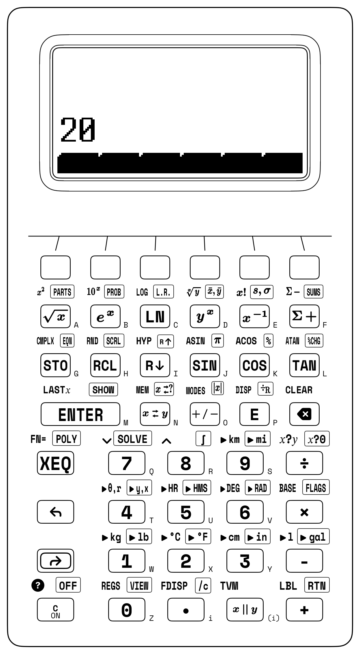
Here Register \(Z\) acts as an optical relay station between the objective and the eyepiece—just as it holds the circular orbital velocity \(v_{\text{orb},1}\) in a Hohmann orbital transfer while the vis-viva perigee speed \(v_p = \sqrt{\mu_\oplus(2/r_1 - 1/a)}\) assembles in Registers \(Y\) and \(X\). When solving a single-stage Gaussian thin-lens equation such as \(\frac{1}{f} = \frac{1}{30} + \frac{1}{60}\) from positive object and image distances, the harmonic parallel operator yields \(f = 30 \parallel 60 = \mathbf{20\text{ cm}}\) directly (Figure 13.2).
13.3.3 Try It on the Stack
- Reynolds Regime & Root-Sum-Square (RSS) Tolerance Stackup: First, verify that blood plasma (\(\rho = 1,025\text{ kg/m}^3,\; \mu = 1.5 \times 10^{-3}\text{ Pa}\cdot\text{s}\)) flowing through a \(D = 0.004\text{ m}\) vessel at \(v = 0.45\text{ m/s}\) lies in the laminar regime by evaluating \(\text{Re} = \rho v D / \mu = \mathbf{1,230} < 2,300\); second, for three mated machined bearing spacers carrying independent bilateral \(3\sigma\) tolerances of \(t_1 = \pm 0.04\text{ mm}\), \(t_2 = \pm 0.03\text{ mm}\), and \(t_3 = \pm 0.12\text{ mm}\), evaluate the statistical assembly tolerance \(t_{\text{RSS}} = \sqrt{t_1^2 + t_2^2 + t_3^2}\) and compare it against the worst-case sum \(0.19\text{ mm}\). (Verified Register \(X\) results: \(\text{Re} = \mathbf{1,230}\) and \(t_{\text{RSS}} = \mathbf{0.13\text{ mm}}\).)
- Gauss Thin-Lens Focal Length via Parallel Operator: An optical bench places an illuminated reticle \(d_o = 30\text{ cm}\) in front of a converging singlet that focuses a sharp real image at \(d_i = 60\text{ cm}\) behind the lens. Combine \(30\) and \(60\) with the harmonic parallel operator to solve \(\frac{1}{f} = \frac{1}{d_o} + \frac{1}{d_i}\). (Verified Register \(X\) result: \(f = \mathbf{20\text{ cm}}\).)
- 10 dB Matched Bridged-T Attenuator Synthesis: For an \(A_{\text{dB}} = 10\text{ dB}\) attenuator on a \(Z_0 = 600\,\Omega\) studio transmission line (\(K = 10^{10/20} \approx 3.162\)), multiply \(K - 1 \approx 2.162\) by \(Z_0 = 600\) to form the series bridge resistor \(R_1 = Z_0(K - 1)\) in Register \(X\), then enter \(Z_0 = 600\) (lifting \(R_1\) to Register \(Y\)), restore \(K - 1\) via
LASTX, and divide to obtain the shunt resistor \(R_2 = Z_0/(K - 1)\). (Verified stack result: \(Y = R_1 \approx \mathbf{1,297.367\,\Omega}\) and \(X = R_2 \approx \mathbf{277.485\,\Omega}\).)