Chapter 12: Curve Profiling, Composite Mensuration & Structural Mechanics
In 1637, the French philosopher and mathematician René Descartes introduced the coordinate system that united algebra and geometry in La Géométrie (Descartes, 1637). For nearly two millennia before Descartes, synthetic geometry and symbolic algebra had existed as two separate intellectual worlds: geometric figures—circles, parabolas, and mechanical curves—were studied visually through compass-and-straightedge constructions, while algebraic equations were treated as numerical recipes yielding isolated numbers stripped of spatial form. Before trusting any single root, definite integral, or regression slope, however, an analyst needs to see the global behavior of an equation at once—where its roots cross zero, where its peaks and valleys bend, and how a structural cross-section distributes material around its balance axis.
Legend relates that while lying in bed one morning watching a fly crawl across the coffered ceiling tiles of his room, Descartes realized that the insect's instantaneous position in the plane was uniquely specified by two perpendicular distances measured from two fixed reference edges of the ceiling. By laying down a horizontal reference axis of abscissas (\(x\)) and a vertical axis of ordinates (\(y\)) intersecting at an origin \((0, 0)\), Descartes established a one-to-one correspondence between spatial geometry and symbolic algebra: * Every point \(P\) in the plane corresponds to an ordered pair of real numbers \((x, y)\), pairing the abscissa \(x\) in Register \(X\) with the ordinate \(y\) in Register \(Y\). * Every algebraic function \(y = f(x)\) defines a continuous geometric locus—a curve swept out in space as the independent coordinate \(x\) varies across an operating domain \([a, b]\). * Every geometric intersection, tangent peak, inflection point, or enclosed planar area corresponds to an algebraic root \(f(x) = 0\), a vanishing first derivative \(f'(x) = 0\), a vanishing second derivative \(f''(x) = 0\), or a definite integral \(\int_a^b f(x)\,dx\).
Across engineering analysis—whether profiling the interatomic potential well of a diatomic molecule, tracing the sag of a suspension bridge cable, locating the neutral axis and bending moment of inertia of a perforated steel girder, or auditing experimental load-cell residuals against a deflected beam span—this correspondence turns visual form into quantitative structure.
12.1 Coordinate Topology, Extrema & Interatomic Potential Wells
Before applying numerical root-finding or definite integration to an unfamiliar physical law, an experienced analyst builds a clear mental picture of the curve's shape across its operating window \([x_{\min}, x_{\max}]\).
12.1.1 The Anatomy of a Curve: Roots, Peaks, Inflections, and the Kissing Circle
Four geometric landmarks govern the behavior of any smooth curve \(y = f(x)\). The first landmark is its zero crossings and curve intersections (\(f(x) = 0\)), marking where a structural beam's internal bending moment changes sign, where the net force between two atoms vanishes, or where two trajectories \(g(x)\) and \(h(x)\) cross. Subtracting the two curves forms a single vertical gap function \(f(x) = g(x) - h(x)\) whose roots \(f(x^*) = 0\) mark the exact coordinates of intersection (Brent, 1973).
The second landmark is the curve's local peaks (maxima) and valleys (minima) (\(f'(x) = 0\)). As you climb over the crest of a hill or walk across the floor of a valley, the ground beneath your feet becomes momentarily flat (\(f'(x^*) = 0\)). By sampling the curve at a small symmetric step size \(h\) to the left (\(x - h\)) and right (\(x + h\)) of \(x\)—which cancels odd-order Taylor terms to leave only a tiny quadratic truncation error \(\mathcal{O}(h^2)\)—we can evaluate both the first derivative \(f'(x)\) and the second derivative \(f''(x)\) to distinguish a peak from a valley without drawing the entire graph:
Across the symmetric interval \([x - h, x + h]\), the secant slope divides the net vertical rise \(f(x + h) - f(x - h)\) by the total horizontal span \(2h\), while the second difference \(f(x + h) - 2f(x) + f(x - h) = [f(x + h) - f(x)] - [f(x) - f(x - h)]\) compares the two flanking heights \(f(x + h) + f(x - h)\) against twice the midpoint height \(2f(x)\) over \(h^2\). At a stationary point where \(f'(x^*) = 0\), a negative second derivative (\(f''(x^*) < 0\)) means both neighbors sit below the midpoint so the curve arches downward like an umbrella (a local maximum), whereas a positive second derivative (\(f''(x^*) > 0\)) means both neighbors sit above the midpoint so the curve cups upward like a bowl (a local minimum).
The third landmark is the curve's inflection points and curvature transitions (\(f''(x) = 0\)). Along an S-shaped mountain road that curves to the right and then bends to the left, the steering wheel passes through straight-ahead center at the exact instant the vehicle crosses from the right-hand bend into the left-hand bend. That transition point where a curve reverses concavity (\(f''(x) = 0\)) is an inflection point, marking the point of steepest tangent slope on an S-shaped response curve, the point of maximum restoring tension in a stretched chemical bond, or the point of zero bending moment along a deflected structural beam.
For any cubic polynomial \(f(x) = ax^3 + bx^2 + cx + d\), differentiating twice gives \(f''(x) = 6ax + 2b = 0\), placing the unique inflection point at \(x_{\text{infl}} = -b/(3a)\)—midway between the cubic's local peak and local valley. On the cubic response curve \(f(x) = x^3 - 6x^2 + 9x + 1\), whose slope \(f'(x) = 3(x - 1)(x - 3)\) vanishes at a local maximum \((1, 5)\) and a local minimum \((3, 1)\), the inflection point sits halfway between them at \((2, 3)\).
The fourth landmark is the osculating radius of curvature (\(\rho\)). To measure how sharply a road or trajectory bends at any given point \((x, f(x))\), the osculating circle ("kissing circle") is defined as the unique circle sharing both the curve's tangent slope \(f'(x)\) and its second derivative \(f''(x)\) at that point. Its radius is the Radius of Curvature \(\rho(x)\), and its reciprocal \(\kappa(x) = 1/\rho(x)\) is the geometric curvature:
Because \(|f''(x)|\) tracks how fast the slope changes per unit of horizontal step \(dx\), whereas geometric curvature measures how fast the tangent angle turns per unit of arc length \(ds = \sqrt{1 + (f'(x))^2}\,dx\) along the tilted curve itself, a steep grade \(f'(x)\) stretches a longer arc path \(ds\) across each horizontal unit \(dx\) and dilutes the bend by the factor \(\bigl[1 + (f'(x))^2\bigr]^{3/2}\).
When a train or automobile travels at speed \(v\) along a curve of radius \(\rho\), passengers feel a sideways centripetal acceleration \(a_c = v^2/\rho\). If a civil engineer joined a straight highway tangent (\(\kappa = 0,\; \rho = \infty\)) abruptly to a circular turn of radius \(R\) (\(\kappa = 1/R\)), the lateral acceleration would jump from zero to \(v^2/R\) at the tangent point, jerking the steering wheel in the driver's hands. Highway and railway engineers therefore insert a Clothoid Transition Spiral of total transition ramp length \(L_s\) and clothoid scale constant \(A = \sqrt{R L_s}\), governed by \(\rho(s) \cdot s = A^2 = R L_s\), along which the local radius \(\rho(s)\) shrinks inversely with arc distance \(s\) from the tangent entry so curvature \(\kappa(s) = s/(R L_s)\) ramps up linearly from \(0\) to \(1/R\) as you turn the steering wheel at a smooth, constant rate. On a parabolic vertical highway crest curve \(y(x) = -2.5 \times 10^{-3} x^2 + 0.04 x + 100\) (\(y'' = -0.005\text{ m}^{-1}\)) at station \(x = 4\text{ m}\) where the grade is \(y'(4) = +0.02\) (\(+2\%\)), the factor \([1 + (0.02)^2]^{1.5} \approx 1.001\) divided by \(|y''| = 0.005\text{ m}^{-1}\) gives an osculating radius of curvature of \(\rho(4) \approx \mathbf{200.12\text{ m}}\).
12.1.2 Interatomic Potential Wells, Critical Isotherms & Wave Envelopes
On a \(132 \times 65\) display, every steep wall, valley floor, and inflection knee of a plotted physical law reflects a balance between competing physical terms.
Atomic Repulsion vs. Dispersion Attraction — The Lennard-Jones \((12, 6)\) Potential Well: Ordinary matter avoids both collapsing into a dense point and flying apart into an ideal gas because of the balance between short-range repulsion and long-range attraction. When two electrically neutral argon atoms approach each other from a center-to-center distance \(r\), fleeting quantum fluctuations in their electron clouds induce synchronized electric dipoles (the dispersion force), pulling the atoms together with a gentle attractive potential proportional to \(-(\sigma/r)^6\). Once the atoms come closer than their collision diameter \(\sigma\) (where the potential crosses zero), however, their electron shells begin to overlap and quantum exclusion erects a fierce repulsive barrier that climbs as the twelfth power \(+(\sigma/r)^{12}\). Scaling the bracket by four times the potential well depth \(\varepsilon\)—the minimum binding energy needed to pull an equilibrium pair of atoms apart—defines the Lennard-Jones \((12, 6)\) Potential \(V(r)\) and the interatomic force \(F(r) = -dV/dr\):
Choosing the prefactor \(4\varepsilon\) normalizes the bracket so that when \((\sigma/r)^6 = 1/2\), the valley floor reaches \(-\varepsilon\), while differentiating with respect to \(r\) raises both inverse powers by one to pit an outward \(+(\sigma/r)^{13}\) repulsive push against an inward \(-(\sigma/r)^7\) attractive pull in \(F(r)\). This competition between an inverse twelfth power and an inverse sixth power carves an asymmetric potential well defined by four geometric landmarks. At short range (\(r < \sigma\)), raising a fraction larger than \(1\) to the twelfth power dwarfs the sixth power, sending \(V(r)\) shooting nearly straight up toward \(+\infty\) along a steep repulsive wall that gives solid matter its rigidity. At the exact collision root (\(r = \sigma\)), both \((\sigma/r)^{12}\) and \((\sigma/r)^6\) equal \(1\) and cancel out, producing the zero crossing \(V(\sigma) = 0\).
Slightly beyond \(\sigma\), the inward attraction and outward repulsion balance (\(F(r_{\min}) = 0\)) at the equilibrium bond valley (\(r_{\min} = 2^{1/6}\sigma \approx 1.122\,\sigma\)), where \(V(r_{\min}) = -\varepsilon\); substituting \(u = (\sigma/r)^6\) collapses the twelfth-degree rational curve into the simple parabola \(V(u) = 4\varepsilon u(u - 1)\), whose vertex sits halfway between \(u = 0\) and \(u = 1\) at \(u = 1/2\). Finally, as two atoms are pulled apart from the valley floor, their restoring attraction initially grows stronger—like stretching a spring—until their separation reaches the inflection fracture limit (\(r_{\text{infl}} = (26/7)^{1/6}\sigma \approx 1.244\,\sigma\)) where \(V''(r_{\text{infl}}) = 0\). Beyond this inflection distance, the restoring force weakens with further stretching: the atomic bond necks down and snaps, and \(V(r)\) levels off asymptotically toward zero.
The macroscopic van der Waals equation of state \(\bigl(P + a/V_m^2\bigr)(V_m - b) = RT\) is the thermodynamic mirror of the Lennard-Jones potential well: the excluded-volume constant \(b\) comes from the hard repulsive wall at \(r < \sigma\), while the cohesion pressure \(a/V_m^2\) comes from the attractive \(-(\sigma/r)^6\) tail.
A plot of pressure \(P(V_m) = \frac{RT}{V_m - b} - \frac{a}{V_m^2}\) against molar volume \(V_m\) traces the geometry of a phase transition. Below the critical temperature \(T_c = \frac{8a}{27Rb}\), the attractive \(-a/V_m^2\) dip carves an S-shaped cubic wiggle (a local minimum followed by a local maximum) across the two-phase liquid–vapor region, where boiling water and steam coexist at constant vapor pressure. As we warm the fluid toward \(T_c\), the local peak and local valley of the S-curve move closer together until, along the critical isotherm \(T = T_c\), they merge into a single horizontal inflection point where both the first and second volume derivatives vanish, fixing the critical molar volume \(V_{m,c}\), the critical pressure \(P_c\), and the dimensionless critical compressibility factor \(Z_c\):
Simultaneously solving the vanishing slope and vanishing curvature conditions shows that at the critical point, molecules are packed until the molar volume \(V_{m,c} = 3b\) is exactly three times the excluded hard-sphere volume \(b\), while the critical pressure \(P_c = a/(27b^2)\) scales directly with intermolecular cohesion \(a\) and inversely with \(b^2\). Combining \(P_c\), \(V_{m,c}\), and \(T_c = \frac{8a}{27Rb}\) cancels both fluid-specific constants \(a\) and \(b\) to yield the universal critical compressibility ratio \(Z_c = \frac{P_c V_{m,c}}{R T_c} = \frac{3}{8} = 0.375\), showing that intermolecular attraction compresses a van der Waals fluid at its critical point to \(37.5\%\) of the volume predicted by the ideal gas law (\(P V_m / R T = 1\)). Above \(T_c\), the inflection knee straightens out so the slope \(\partial P/\partial V_m\) is negative everywhere, and liquid and gas merge into a single supercritical fluid.
Two modulated-envelope laws and one harmonic series round out these curve families. Whenever a rapid carrier oscillation is multiplied by a slowly decaying envelope, the outer envelope curves touch every oscillation peak. In an automotive shock absorber \(y(t) = e^{-\zeta\omega_n t}\cos(\omega_d t)\) with decay rate \(\zeta\omega_n = 0.4\text{ s}^{-1}\) and oscillation frequency \(\omega_d = 3\text{ rad/s}\) at \(t = 0.8\text{ s}\), the cosine carrier \(\cos(2.4\text{ rad}) \approx -0.737\) attenuated by the exponential envelope \(e^{-0.32} \approx 0.726\) gives an instantaneous displacement of \(y(0.8) \approx \mathbf{-0.535\text{ m}}\). In a single-slit Fraunhofer optical diffraction pattern \(I(x) = I_0\operatorname{sinc}^2(x) = I_0\bigl(\frac{\sin x}{x}\bigr)^2\), dividing \(\sin(1.2\text{ rad}) \approx 0.932\) by its radian argument \(1.2\) gives field amplitude \(\operatorname{sinc}(1.2) \approx \mathbf{0.777}\) and relative intensity \(I/I_0 \approx \mathbf{0.603}\) inside the central bright fringe (\(|x| < \pi\)).
Even a discontinuous, sharp-cornered square wave can be synthesized as a Fourier series of smooth odd sine harmonics \(\frac{4}{\pi}\sum_{k=1}^N \frac{\sin((2k-1)x)}{2k-1}\). Summing just the first three odd harmonics \(\sin x + \frac{1}{3}\sin(3x) + \frac{1}{5}\sin(5x)\) at \(x = 0.5\text{ rad}\) yields \(0.479 + 0.332 + 0.12 \approx \mathbf{0.932}\) (which scales by \(4/\pi\) to \(\approx 1.186\)), and adding higher harmonics reveals two narrow "ears" near each jump discontinuity that overshoot the flat roof by \(\approx 8.95\%\) of the peak-to-peak jump (\(\approx 17.9\%\) above the unit plateau)—the Gibbs phenomenon.
The distribution of weight along a flexible cable of horizontal tension \(H\) suspended between two towers explains why two distinct structural curves arise: when weight \(w\) is distributed uniformly per unit horizontal span \(dx\)—as on a suspension bridge where vertical steel hanger rods support a flat horizontal roadway—the cable slope \(\frac{dy}{dx} = \frac{wx}{H}\) integrates to an exact parabola \(y = h_0 + \frac{4f}{L^2}x^2\). On a suspension cable of span \(L = 64\text{ m}\), mid-span sag \(f = 16\text{ m}\) (\(4f/L^2 = 1/64 \approx 0.016\text{ m}^{-1}\)), and clearance \(h_0 = 2\text{ m}\), the vertical suspender rods have length \(\frac{1}{64}(12^2) + 2 = \mathbf{4.25\text{ m}}\) at station \(x = 12\text{ m}\) and \(\mathbf{11\text{ m}}\) at \(x = 24\text{ m}\).
When a bare power transmission line instead hangs under its own weight per unit arc length \(ds = \sqrt{1 + (dy/dx)^2}\,dx\), the steeper sections near the towers carry more cable weight per horizontal meter than the flat bottom. Solving the differential equilibrium \(\frac{d^2 y}{dx^2} = \frac{w}{H}\sqrt{1 + (dy/dx)^2}\) shows that the bare cable forms a hyperbolic cosine catenary \(y(x) = a\cosh(x/a)\) with parameter \(a = H/w\). For a power line with \(a = 500\text{ m}\) spanning \(L = 200\text{ m}\) (half-span ratio \(\frac{L}{2a} = 0.2\)), the exact catenary sag is \(f_{\text{sag}} = a[\cosh(L/2a) - 1] = 500(\cosh 0.2 - 1) \approx \mathbf{10.033\text{ m}}\) and the true conductor arc length is \(s_{\text{arc}} = 2a\sinh(0.2) \approx \mathbf{201.336\text{ m}}\) (\(\approx 1.336\text{ m}\) of slack beyond the \(200\text{ m}\) tower spacing).
12.2 Composite Cross-Sections, Neutral Axes & Structural Beams
Where land surveyors determine the area and centroid of polygonal parcels from boundary vertices, structural and mechanical engineers find the area, balance point (centroid), and bending stiffness of load-bearing beams and gusset plates built by welding together rectangles and triangles while drilling out circular bolt holes and pipe cutouts.
12.2.1 Additive and Subtractive Planimetry, Centroids & Solids of Revolution
Every complex structural cross-section can be dissected into \(m\) elementary shapes (\(k = 1, 2, \dots, m\)) whose individual areas \(A_k\), local balance points \((x_k, y_k)\), and local bending inertias \(I_{c,k}\) are known from basic geometry (Figure 12.1). Summing the signed piece areas yields the net cross-sectional area \(A_{\text{net}}\), and balancing the area moments locates the composite centroid \((\bar{x}, \bar{y})\):
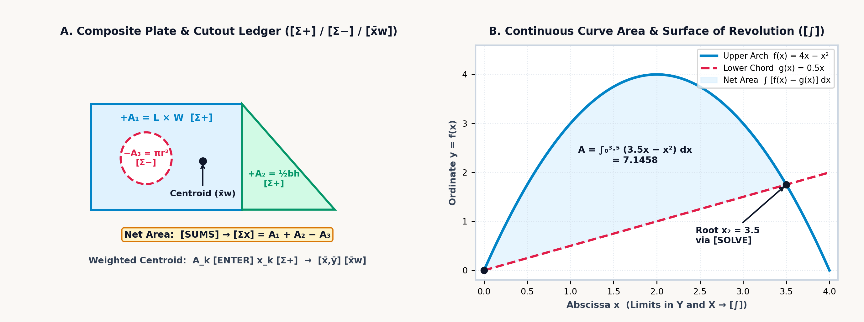
Physically, the composite balance point \((\bar{x}, \bar{y})\) is the area-weighted average of the individual piece centers \((x_k, y_k)\): each solid plate contributes a positive first moment \(+A_k x_k\), any cutout hole or window enters with a negative area \(-A_k\) to deduct the missing metal's torque, and scaling the net moment by the surviving cross-sectional area \(A_{\text{net}} = \sum \pm A_k\) locates the single coordinate pair where the perforated plate balances flat. Five classical building blocks cover nearly every engineering cross-section:
| Geometric Primitive | Area Formula (\(A_k\)) | Centroid Offset from Base/Corner | Second Moment \(I_{xc}\) About Own Centroid |
|---|---|---|---|
| Rectangle (\(b \times h\)) | \(b h\) | \(\bar{x} = \frac{b}{2},\quad \bar{y} = \frac{h}{2}\) | \(I_{xc} = \frac{b h^3}{12}\) |
| Right Triangle (\(b \times h\)) | \(\frac{1}{2} b h\) | \(\bar{x} = \frac{b}{3},\; \bar{y} = \frac{h}{3}\) from \(90^\circ\) corner | \(I_{xc} = \frac{b h^3}{36}\) |
| Full Circle (radius \(r\), diam \(d\)) | \(\pi r^2 = \frac{\pi}{4} d^2\) | \((\bar{x}, \bar{y}) = (x_c, y_c)\) | \(I_{xc} = \frac{\pi r^4}{4} = \frac{\pi d^4}{64}\) |
| Semicircle (radius \(r\) on flat base) | \(\frac{1}{2}\pi r^2\) | \(\bar{y} = \frac{4r}{3\pi} \approx 0.424\,r\) | \(I_{xc} = \left(\frac{\pi}{8} - \frac{8}{9\pi}\right) r^4 \approx 0.11\,r^4\) |
| Parabolic Arch Segment (\(b \times h\)) | \(\frac{2}{3} b h\) | \(\bar{y} = \frac{2}{5} h\) from flat base (\(\frac{3}{5}h\) from vertex) | \(I_{xc} = \frac{8}{175} b h^3\) |
Archimedes' parabolic quadrature law (\(A_{\text{parabola}} = \frac{2}{3}bh\), where the arch occupies two-thirds of its bounding rectangle and the outer spandrel corners occupy the remaining one-third, \(A_{\text{spandrel}} = \frac{1}{3}bh\)) evaluates hull waterplane sections and masonry culvert arches. For a parabolic highway culvert arch of base span \(b = 9\text{ m}\) and crown rise \(h = 4\text{ m}\), the cross-sectional flow area is \(\frac{2}{3}(9)(4) = \mathbf{24\text{ m}^2}\) with centroid height \(\bar{y} = \frac{2}{5}(4) = \mathbf{1.6\text{ m}}\) above the flat invert.
In a composite steel gusset plate of width \(b = 120\text{ mm}\) and height \(h = 80\text{ mm}\) (\(A_1 = 9,600\text{ mm}^2\), centered at \(x_1 = 60\text{ mm}\)) pierced off-center at \(x_2 = 85\text{ mm}\) by a circular pipe cutout of radius \(r = 20\text{ mm}\) (\(A_2 = 400\pi \approx 1,256.637\text{ mm}^2\)), subtracting the hole leaves a net steel area of \(A_{\text{net}} = 9,600 - 400\pi \approx \mathbf{8,343.363\text{ mm}^2}\). Because metal was removed from the right side of the plate (\(x_2 = 85\text{ mm} > 60\text{ mm}\)), the balance point shifts leftward to \(\bar{x} \approx \frac{9,600(60) - 1,256.637(85)}{8,343.363} \approx \mathbf{56.235\text{ mm}}\).
By the Pappus–Guldinus Centroid Theorem, when a planar cross-section of net area \(A_{\text{net}}\) and area centroid distance \(\bar{r}\) (composed of sub-shapes \(k\) with areas \(\pm A_k\) at radial centroid distances \(r_k\))—or a planar curve of arc length \(s\) and arc-centroid distance \(\bar{r}_s\)—is revolved through a full circle about a coplanar axis that does not intersect its interior, the swept surface area \(S\) and volume \(V\) equal:
The geometric intuition is direct: the swept surface area \(S\) or volume \(V\) equals the generating cross-section's arc length \(s\) or net area \(A_{\text{net}}\) multiplied by the circular path circumference \(2\pi\bar{r}_s\) or \(2\pi\bar{r}\) traveled by its centroid during one full revolution—or equivalently, the sum of the individual volumes \(2\pi(\pm A_k)r_k\) swept by each sub-shape \(k\) at its own centroid radius \(r_k\). Thus, revolving our perforated \(120 \times 80\text{ mm}\) gusset cross-section (whose net first moment of area is \(\bar{x}A_{\text{net}} \approx \mathbf{469,185.85\text{ mm}^3}\)) around the \(y\)-axis (\(x = 0\)) generates a machined steel ring with a circular cooling channel of volume \(V = 2\pi\bar{x}A_{\text{net}} \approx \mathbf{2.948 \times 10^6\text{ mm}^3}\) (\(\approx \mathbf{2,947.98\text{ cm}^3}\)).
12.2.2 Why Beams Are Shaped Like an "I": Parallel-Axis Inertia, Elastic Sag, and Model Audits
Structural steel girders are rolled into the shape of an I-beam (with wide top and bottom flanges separated by a thin vertical web) rather than cast as a solid rectangular bar of the same weight because of how bending stress distributes across a cross-section.
When a horizontal beam sags under an internal bending moment \(M\), its top fibers are squeezed in compression while its bottom fibers are stretched in tension. Somewhere between the top and bottom lies a horizontal plane that neither stretches nor compresses—the neutral axis, which passes through the cross-section's area centroid \(\bar{y}\). Under Euler–Bernoulli flexure, the longitudinal bending stress \(\sigma_x(y) = -M y / I_x\) (for vertical coordinate \(y\) measured upward from \(\bar{y}\)) grows linearly with distance \(y\) from that neutral axis, meaning material sitting near the middle of the beam (\(y \approx 0\)) barely helps resist the bending moment \(M\). A beam's resistance to bending is measured by its Second Moment of Area (Area Moment of Inertia, \(I_x = \iint_A y^2\,dA\)). By the Parallel-Axis Theorem (Steiner's theorem), when a rectangular sub-shape \(k\) of width \(b_k\), height \(h_k\), area \(A_k = b_k h_k\), and local centroidal inertia \(I_{c,k} = \frac{b_k h_k^3}{12}\) is shifted by a vertical distance \(d_k = |y_k - \bar{y}|\) away from the composite neutral axis, its contribution to total stiffness equals its own local inertia \(I_{c,k}\) plus its area \(A_k\) multiplied by the square of the transfer distance \(d_k\):
Each sub-shape contributes both its own local bending stiffness \(I_{c,k} = \frac{b_k h_k^3}{12}\) about its mid-plane \(y_k\) and a parallel-axis transfer term \(A_k d_k^2 = A_k(y_k - \bar{y})^2\) measuring the leverage gained by moving that area a distance \(d_k\) away from the composite neutral axis \(\bar{y}\). Because \(A_k d_k^2\) grows with the square of distance from the neutral axis, concentrating the steel into two wide flanges at the top and bottom of an I-beam puts the metal where it works hardest. In a symmetric welded steel I-beam of total depth \(H = 200\text{ mm}\) built from two \(100 \times 20\text{ mm}\) flanges (\(A_f = 2,000\text{ mm}^2\) each, centered at \(d_f = 90\text{ mm}\) from the neutral axis) and a \(10 \times 160\text{ mm}\) web (\(d_w = 0\)), the two transfer terms \(2 \times 2,000(90)^2 = 3.24 \times 10^7\text{ mm}^4\) supply over \(90\%\) of the girder's total moment of inertia \(I_x \approx \mathbf{3.595 \times 10^7\text{ mm}^4}\).
When a beam is asymmetric from top to bottom—such as a structural T-beam cast in gray iron or reinforced concrete (materials that are four times stronger in compression than in tension)—the neutral axis \(\bar{y}\) shifts upward toward the heavy top flange. In a T-beam of total height \(H = 150\text{ mm}\) formed by a \(20 \times 120\text{ mm}\) vertical stem (\(A_1 = 2,400\text{ mm}^2,\; y_1 = 60\text{ mm},\; I_{c,1} = 2.88 \times 10^6\text{ mm}^4\)) and a \(120 \times 30\text{ mm}\) top flange (\(A_2 = 3,600\text{ mm}^2,\; y_2 = 135\text{ mm},\; I_{c,2} = 2.7 \times 10^5\text{ mm}^4\)), the area-weighted centroid sits at \(\bar{y} = \mathbf{105\text{ mm}}\) above the bottom of the stem.
With transfer distances \(d_1 = |60 - 105| = 45\text{ mm}\) and \(d_2 = |135 - 105| = 30\text{ mm}\), the parallel-axis theorem yields a composite inertia of \(I_x = 7.74 \times 10^6 + 3.51 \times 10^6 = \mathbf{1.125 \times 10^7\text{ mm}^4}\). Under a sagging bending moment of \(M = 15\text{ kN}\cdot\text{m}\), the short distance to the top fiber (\(c_{\text{top}} = 45\text{ mm}\)) keeps compressive stress down to \(\sigma_{\text{top}} = \mathbf{-60\text{ MPa}}\), while the longer lever arm to the bottom of the stem (\(c_{\text{bot}} = 105\text{ mm}\)) produces \(\sigma_{\text{bot}} = \mathbf{+140\text{ MPa}}\) of tension.
Thin-walled pressure vessels and hollow transmission shafts obey similar geometric scaling laws. In a thin-walled cylindrical tank of radius \(r\), wall thickness \(t \ll r\), and internal pressure \(p\), pressure pushing outward across a diameter \(2rL\) is resisted by two longitudinal wall strips of area \(2tL\), giving circumferential hoop stress \(\sigma_{\text{hoop}} = \frac{pr}{t}\); pressure pushing on the circular end cap \(\pi r^2\) is resisted by the full ring circumference \(2\pi r t\), giving axial stress \(\sigma_{\text{long}} = \frac{pr}{2t} = \frac{1}{2}\sigma_{\text{hoop}}\). Because hoop stress is twice axial stress (for \(r = 0.45\text{ m},\; t = 9\text{ mm},\; p = 2.4\text{ MPa}\), \(\sigma_{\text{hoop}} = \mathbf{120\text{ MPa}}\) vs. \(\sigma_{\text{long}} = \mathbf{60\text{ MPa}}\)), a burst steam pipe, propellant tank, or grilled sausage always splits along a longitudinal seam.
In a hollow circular shaft of outer radius \(r_o\) and inner bore \(r_i\), torsional polar inertia is \(J = \frac{\pi}{2}(r_o^4 - r_i^4)\). Because stiffness scales with the fourth power of radius, boring out the center of a solid shaft to \(r_i = 0.6\,r_o\) removes \(0.6^2 = \mathbf{36\%}\) of its weight while keeping \(1 - 0.6^4 = \mathbf{87.04\%}\) of its torsional stiffness (\(J \approx \mathbf{5.341 \times 10^{-7}\text{ m}^4}\) and surface shear \(\tau_{\max} = T r_o / J \approx \mathbf{84.259\text{ MPa}}\) for an \(r_o = 25\text{ mm},\; r_i = 15\text{ mm}\) steel shaft under \(T = 1,800\text{ N}\cdot\text{m}\)). When that shaft carries both \(\sigma_x = 140\text{ MPa}\) of bending stress and \(\tau_{xy} \approx 84.259\text{ MPa}\) of torsion, the von Mises octahedral distortion-energy criterion combines them as the Euclidean hypotenuse \(\sigma' = \sqrt{\sigma_x^2 + (\sqrt{3}\,\tau_{xy})^2} \approx \mathbf{202.236\text{ MPa}}\) (giving a safety factor of \(\text{FS} = \sigma_y / \sigma' = 415 / \sigma' \approx \mathbf{2.052}\) for AISI 4140 steel with yield strength \(\sigma_y = 415\text{ MPa}\)).
Two integrations of the Euler–Bernoulli beam equation \(EI\,y''(x) = M(x)\) show that elastic beam deflection under a point load \(F\) grows with the cube of span (\(\delta \propto F L^3 / EI\)): doubling a beam's length multiplies its sag eightfold, while supporting both ends (\(\delta_{\text{simple}} = \frac{F L^3}{48 E I} \approx \mathbf{0.186\text{ mm}}\) for a \(1.5\text{ m}\) steel span of flexural rigidity \(EI = 1.701 \times 10^6\text{ N}\cdot\text{m}^2\) under \(F = 4,500\text{ N}\)) makes the span sixteen times stiffer than clamping one end as a free cantilever (\(\delta_{\text{cantilever}} = \frac{F L^3}{3 E I} \approx \mathbf{2.978\text{ mm}}\)). Along the normalized cantilever profile \(y(\xi) = \frac{1}{2}\xi^2(3 - \xi)\), the mid-span sag at \(\xi = x/L = 0.5\) is \(\mathbf{5/16}\) (\(\approx \mathbf{0.313}\) of tip deflection). When a crane wheel load turns on abruptly at an interior point \(x = a\), the Macaulay singularity bracket \(\langle x - a \rangle^n = (x - a)^n \cdot [x > a]\)—which multiplies the smooth polynomial \((x - a)^n\) by a boolean Heaviside indicator \([x > a]\) that evaluates to \(0\) for \(x \le a\) and \(1\) for \(x > a\)—allows the entire discontinuous beam to be integrated and plotted as a single continuous equation.
Just as integrating bending curvature along a span \(L\) determines elastic deflection, integrating a cross-sectional area \(A(x)\) that tapers continuously along a span \(L\) determines three-dimensional structural and earthwork volume. For any solid whose cross-sectional area \(A(x)\) varies up to a cubic polynomial along length \(L\), Simpson's Prismoidal Formula gives the exact volume as \(V_{\text{prismoid}} = \frac{L}{6}(A_1 + 4A_m + A_2)\), weighting the two end areas \(A_1, A_2\) and four times the mid-span area \(A_m\). When an \(L = 30\text{ m}\) highway cut tapers in width and depth from \(A_1 = 24\text{ m}^2\) through mid-section \(A_m = 45.5\text{ m}^2\) to \(A_2 = 76\text{ m}^2\), naive average-end-area billing \(\frac{L}{2}(A_1 + A_2) = \mathbf{1,500\text{ m}^3}\) overestimates the true prismoidal volume \(\mathbf{1,410\text{ m}^3}\) by \(\mathbf{90\text{ m}^3}\).
Once a structural beam or load cell is placed under test in the laboratory, residual analysis verifies whether a linear calibration model \(\hat{y} = mx + b\) fits the measured deflection data or hides a nonlinear bend. The 1973 diagnostic benchmark Anscombe's Quartet consists of four datasets of \(n = 11\) points that share the identical mean, variance, regression line \(\hat{y} = 3 + 0.5x\), and correlation coefficient \(r \approx 0.816\), even though Dataset I is a healthy linear cloud, Dataset II is a curved parabola, Dataset III contains a corrupted outlier spike, and Dataset IV is skewed by a single high-leverage endpoint. Before trusting a high correlation \(r\), always check the residuals \(e_k = y_k - \hat{y}(x_k)\): if they alternate signs randomly, the linear fit is sound; if they display a systematic sign run (\(+, -, +\) or \(-, +, +, -\)), your physical system contains unmodeled curvature \(f''(x) \ne 0\).
12.3 Stack Patterns for Curve Profiling & Structural Cross-Sections
Curve profiling, composite-section planimetry, and prismoidal volume audits rely on three evaluation patterns across the four-level stack (T, Z, Y, X):
- Companion App Function & Scatter Plotting (
[↱] [PLOT]), Relational Step Indicators (x?y,x?0), & Top-Register Replication ([ENTER] [ENTER] [ENTER]): In the companion app, pressing[↱] [PLOT](right-shifted on[x∥y]; omitted from physical firmware for exam compliance) opens the graphicalPLOTworkspace. When equations are stored in[↱] [EQN], the softkeys display the available equation variables (A–Z) to plot across \([x_{\min}, x_{\max}]\) in \((Y, X)\) (defaulting to \([-3, 3]\) when \(Y = X\), or \([-10, 10]\) when executed via[XEQ]). When[Σ+]statistical data is present and no equations are stored (CLEQN), pressing[↱] [PLOT]renders a 1-Var or 2-Var scatter plot directly without aSTATsoftkey. Inside[↱] [EQN], relational testsx?yandx?0on[÷]return1when true and0when false so Macaulay brackets \(\langle X - A \rangle = (X - A)\cdot [X > A]\) graph as a single equation, while the 101-point canvas highlights roots or shades integrals from[↱] [SOLVE]or[↱] [∫]and supports pan (<,>) and zoom (OUT,IN). For numeric sweeps at \(x\), pressing[ENTER]three times fills all four levels (T = Z = Y = X = x) so[×]replenishes \(x\) from \(T\) across Horner stages, and[↱] [POLY]extracts closed-form cubic roots and inflection points. - Subtractive Planimetry & Weighted Centroids (
[Σ+],[↰] [Σ-],[↱] [SUMS],[↱] [x̄,ȳ]): After resetting the six statistical accumulators (R28–R33) to0via[↰] [CLEAR]\(\to\)CLSTAT([CLΣ]), staging each solid sub-area \(A_k\) (the weight) in Register \(Y\) and its centroid coordinate \(x_k\) in Register \(X\) before pressing[Σ+]—and staging any cutout hole's positive area \(A_{\text{hole}}\) in Register \(Y\) and center \(x_{\text{hole}}\) in Register \(X\) before pressing[↰] [Σ-](left-shifted on[Σ+])—accumulates net area inΣy([↱] [SUMS]\(\to\)Σy), net first moment inΣxy([↱] [SUMS]\(\to\)Σxy), and composite centroid \(\bar{x} = \Sigma xy / \Sigma y\) inx̄w([↱] [x̄,ȳ]\(\to\)x̄w). - Regression Residual Auditing (
[↱] [L.R.]\(\to\)ŷ): After logging calibration pairs \((Y = y_k,\; X = x_k)\) with[Σ+], entering a test abscissa \(x_k\) and tapping[↱] [L.R.](right-shifted on[LN]) \(\to\)ŷplaces the linear prediction \(\hat{y}(x_k)\) in Register \(X\) (whilerin[↱] [L.R.]queries Pearson's correlation coefficient \(r\)); keying the measured ordinate \(y_k\) and pressing[x⇄y] [-]isolates the residual \(e_k = y_k - \hat{y}(x_k)\).
12.3.1 T-Register Replication for Cubic Inflection & Curve Profiling
Whenever you need to evaluate a polynomial \(f(x)\) (or both \(f(x)\) and its shifted derivative core) at a target station \(x\), filling all four stack registers (T = Z = Y = X = x) turns Register \(T\) into a permanent supply of \(x\). Because every dyadic multiplication drops the stack and copies Register \(T\) into Register \(Z\), \(x\) stays parked in Register \(Y\) ready for the next Horner stage without being typed a second time.
To profile the cubic response curve \(f(x) = x^3 - 6x^2 + 9x + 1 = ((x - 6)x + 9)x + 1\) at its inflection abscissa \(x_{\text{infl}} = 2\), replicating \(2\) across all four stack levels (T = Z = Y = X = 2) and subtracting \(6\) forms the innermost Horner binomial \(x - 6 = -4\) in Register \(X\). Multiplying by \(x = 2\) waiting in Register \(Y\) (while Register \(T\) replenishes \(2\) into Register \(Z\)) and adding \(9\) yields \((x - 6)x + 9 = 1\), after which a second multiplication by \(x = 2\) from Register \(Y\) and addition of \(1\) delivers the inflection ordinate \(y_{\text{infl}} = f(2) = \mathbf{3}\) in Register \(X\) with \(x = 2\) still preserved in Registers \(T, Z,\) and \(Y\).
Once \(x = 2\) is swapped from Register \(Y\) back into Register \(X\), evaluating the first derivative yields the inflection tangent slope \(f'(2) = (3x - 12)x + 9 = \mathbf{-3}\) while the second derivative vanishes (\(f''(2) = 6x - 12 = \mathbf{0}\)). That \(T\)-register replication rhythm evaluates any polynomial or repeated-parameter family—whether sweeping horizontal stations \(x = 12\text{ m}, 24\text{ m}\) along a parabolic suspension bridge cable by parking the sag coefficient \(4f/L^2 = 1/64\text{ m}^{-1}\) in Register \(T\), or evaluating van der Waals cubic isotherms across molar volume \(V_m\).
12.3.2 Subtractive Planimetry, Parallel-Axis Inertia & Residual Auditing
To find the net area \(A_{\text{net}}\), composite centroid \(\bar{x}\), and revolved Pappus–Guldinus volume of a plate with cutouts, the statistical accumulators act as a direct planimeter. After clearing the statistical registers (CLSTAT), enter each solid sub-shape's area \(A_k\) in Register \(Y\) (the weight) and its center coordinate \(x_k\) in Register \(X\) for positive accumulation. For any cutout hole, stage its positive area \(A_{\text{hole}}\) in Register \(Y\) and its center \(x_{\text{hole}}\) in Register \(X\) for subtractive accumulation, which deducts both the hole's area and its first moment:
| Keystroke | Register T | Register Z | Register Y | Register X | What Happens on the Stack |
|---|---|---|---|---|---|
[↰] [CLEAR] [CLΣ] |
\(0\) | \(0\) | \(0\) | \(0\) | Clear statistical accumulators (CLSTAT softkey; R28–R33 \(= 0\)) |
120 [ENTER] 80 [×] 60 [Σ+] |
\(0\) | \(0\) | \(9600\) | \(1\) | Accumulate solid rectangle (\(A_1 = 9,600\) in \(Y\), \(x_1 = 60\) in \(X\)) |
20 [↰] [x²] [↱] [π] [×] 85 [↰] [Σ-] |
\(0\) | \(9600\) | \(1256.637\) | \(0\) | Subtract circular cutout (\(A_2 \approx 1,256.637\) in \(Y\), \(x_2 = 85\) in \(X\)) |
[↱] [SUMS] [Σy] |
\(0\) | \(9600\) | \(1256.637\) | \(8343.363\) | Net composite plate area \(A_{\text{net}} = \sum y \approx 8,343.363\text{ mm}^2\) |
[↱] [x̄,ȳ] [x̄w] |
\(9600\) | \(1256.637\) | \(8343.363\) | \(56.235\) | Composite centroid \(\bar{x} = \sum xy / \sum y \approx 56.235\text{ mm}\) |
Because the first-moment accumulator \(\sum (\pm A_k x_k) \approx \mathbf{469,185.85\text{ mm}^3}\) is retained in memory, multiplying that net first moment by \(2\pi\) yields the 3D Pappus–Guldinus revolved ring volume (\(\approx \mathbf{2,947.98\text{ cm}^3}\)) for any axisymmetric flywheel or flanged pipe fitting with arbitrary grooves and bolt holes.
Once the weighted-mean operation locates the neutral axis \(\bar{y}\) of an asymmetric section, that same statistical accumulation feeds into the parallel-axis theorem. On the \(H = 150\text{ mm}\) asymmetric T-beam, accumulating the stem and flange areas with their centroid heights places the composite neutral axis \(\bar{y} = 105\text{ mm}\) in Register \(X\). As you then sum the stem and flange parallel-axis contributions (\(I_1 = 7.74 \times 10^6\text{ mm}^4\) and \(I_2 = 3.51 \times 10^6\text{ mm}^4\)) into the total moment of inertia \(I_x = 1.125 \times 10^7\text{ mm}^4\), automatic stack lift carries \(\bar{y} = 105\text{ mm}\) up into Registers \(T, Z,\) and \(Y\), where it remains visible on the display ready to scale \(M / I_x\) (\(M = 1.5 \times 10^7\text{ N}\cdot\text{mm}\)) into the bottom-fiber tensile stress \(\sigma_{\text{bot}} = +140\text{ MPa}\).
When auditing experimental load-cell calibration points such as \((1\text{ kN}, 2.1\text{ mV})\), \((2\text{ kN}, 3.9\text{ mV})\), and \((3\text{ kN}, 6\text{ mV})\) against Anscombe's Quartet traps, accumulating the \((x_k, y_k)\) pairs into the statistical registers fits the regression line \(\hat{y} = 0.1 + 1.95x\) (\(r \approx 0.999\)). Evaluating the linear-regression prediction \(\hat{y}(x_k)\) at \(x_k = 1, 2, 3\) in Register \(X\) and subtracting each prediction from its measured ordinate \(y_k\) then yields the \(+0.05, -0.1, +0.05\text{ mV}\) residual sign run (\(+, -, + \implies\) upward quadratic bow \(f''(x) > 0\)).
12.3.3 Simpson's Prismoidal Quadrature vs. Average-End-Area Auditing
To compare two competing engineering formulas—such as naive average-end-area earthwork billing \(V_{\text{avg-end}} = \frac{L}{2}(A_1 + A_2)\) versus Simpson's exact Prismoidal Formula \(V_{\text{prismoid}} = \frac{L}{6}(A_1 + 4A_m + A_2)\) for an \(L = 30\text{ m}\) highway cut (\(A_1 = 24\text{ m}^2,\; A_m = 45.5\text{ m}^2,\; A_2 = 76\text{ m}^2\))—the baseline estimate can be evaluated first so automatic stack lift carries it into the upper registers while the exact prismoidal sum is assembled in Registers \(Y\) and \(X\). Forming the average-end-area volume \(\frac{30}{2}(24 + 76) = \mathbf{1,500\text{ m}^3}\) in Register \(X\) and then starting the prismoidal sum \(A_1 + 4A_m = 24 + 4(45.5) = 206\text{ m}^2\) lifts \(V_{\text{avg-end}} = 1,500\text{ m}^3\) into Registers \(T, Z,\) and \(Y\).
Once the far-end area \(A_2 = 76\text{ m}^2\) is added and scaled by \(L/6 = 30/6\), Simpson's prismoidal volume \(V_{\text{prismoid}} = \mathbf{1,410\text{ m}^3}\) sits in Register \(X\) with \(V_{\text{avg-end}} = 1,500\text{ m}^3\) waiting in Register \(Y\); swapping \(X\) and \(Y\) and subtracting reveals the earthwork correction \(\Delta V = V_{\text{prismoid}} - V_{\text{avg-end}} = \mathbf{-90\text{ m}^3}\) from the two values already on the stack. When a section is bounded by intersecting curves \(g(x) = 4 - x^2\) and \(h(x) = x + 2\), storing \(f(x) = 2 - x - x^2\) in EQN lets SOLVE locate the crossings (\(x_1 = -2,\; x_2 = +1\)) and ∫ integrate the enclosed area (\(\int_{-2}^1 f(x)\,dx = 4.5\)).
12.3.4 Try It on the Stack
- Cubic Curve Stationary Points & Inflection Audit: For \(f(x) = x^3 - 12x\), evaluate \(f(-2)\) and \(f(2)\) via Horner's form \((x^2 - 12)x\) to verify its extrema where \(f'(x) = 3x^2 - 12 = 0\), and confirm the inflection point at \(x = 0\). (Verified Register \(X\) results: \(f(-2) = \mathbf{16}\), \(f(0) = \mathbf{0}\), \(f(2) = \mathbf{-16}\).)
- Perforated Plate Centroid via Subtractive Accumulation: An aluminum plate of area \(A_1 = 200 \times 100 = 20,000\text{ mm}^2\) centered at \(x_1 = 100\text{ mm}\) has a square cutout \(A_2 = 50 \times 50 = 2,500\text{ mm}^2\) centered at \(x_2 = 150\text{ mm}\). Accumulate \((Y = 20,000,\; X = 100)\) positively and \((Y = 2,500,\; X = 150)\) subtractively, then read \(\bar{x} = \Sigma xy / \Sigma y\). (Verified Register \(X\) result: \(\bar{x} \approx \mathbf{92.857\text{ mm}}\), net area \(\Sigma y = \mathbf{17,500\text{ mm}^2}\).)
- Symmetric Welded I-Beam Flange Inertia Share: For the \(H = 200\text{ mm}\) steel I-beam with two \(100 \times 20\text{ mm}\) flanges (\(A_f = 2,000\text{ mm}^2\) each at \(d_f = 90\text{ mm}\)) and total inertia \(I_x \approx 3.595 \times 10^7\text{ mm}^4\), evaluate \(2 A_f d_f^2\) and divide by \(I_x\). (Verified Register \(X\) results: \(2A_f d_f^2 = \mathbf{3.24 \times 10^7\text{ mm}^4}\), supplying \(\approx \mathbf{90.1\%}\) of bending stiffness.)