Chapter 11: Percentages, Time Value of Money & Cash-Flow Valuation
In 1202, Leonardo of Pisa (Fibonacci) posed a question in Chapters 12 and 13 of Liber Abaci that founded quantitative finance: If a merchant or sovereign treasury is promised a stream of periodic payments over future years while capital earns compound interest each year, what single lump sum paid today is its exact fair equivalent, and which of two competing cash-flow streams makes the investor wealthier? Silicon registers switch binary states across nanoseconds; economic enterprises commit capital across years and decades, where time itself acts as an exponential multiplier. Before Fibonacci's analysis, medieval bookkeepers routinely confused simple interest, in which interest accrues only on the original principal \(P_0\), with compound interest, in which each period's accrued return is folded back into the principal to earn returns in all subsequent periods.
By discounting each future payment back to the present day through repeated division by the compound growth factor \((1 + i)\), Fibonacci established the first principle of financial economics: a unit of currency promised in the future is not commensurate with a unit of currency held today until both are transported to a common point in time.
11.1 Multiplicative Asymmetry, Compounding & the Five-Variable TVM Balance Law
Fibonacci's present-value discounting principle rests on the time asymmetry of productive capital. A dollar in hand today can be invested at a periodic rate of return \(i\) to grow to \((1 + i)\) dollars one period from now, \((1 + i)^2\) dollars two periods from now, and \((1 + i)^n\) dollars after \(n\) compounding periods. Even in the absence of default risk, inflation erodes purchasing power while opportunity cost rewards productive investment. Moving a sum of money forward in time by \(n\) periods multiplies it by \((1 + i)^n\) (compounding); moving a future cash flow backward in time by \(n\) periods multiplies it by the reciprocal factor \((1 + i)^{-n}\) (discounting).
11.1.1 The Asymmetry of Gain and Loss: Drawdowns, Markups, and Margins
Before introducing time and compounding periods, financial analysis begins with instantaneous proportional scaling: percentages (%), relative changes (%CHG), retail markdowns, and profit margins. Untrained intuition treats percentage changes as additive, yet every percentage adjustment \(r\%\) is a multiplicative scale factor \((1 \pm \delta)\) with fractional change \(\delta = r / 100\).
Suppose an equity portfolio or retail inventory begins with initial capital \(V_0\) and suffers a fractional drawdown \(-\delta\) during a market correction, followed in the next quarter by an equal fractional rebound \(+\delta\) to reach an ending value \(V_{\text{final}}\). By the algebraic identity for the difference of two squares, applying a fractional loss \(-\delta\) and an equal fractional gain \(+\delta\) in either order always leaves a net multiplicative drag of \(-\delta^2\):
Because the initial drawdown shrinks \(V_0\) to a diminished capital base \(V_0(1 - \delta)\), the subsequent rebound \((1 + \delta)\) compounds only against that smaller survivor rather than the original principal, locking in a permanent quadratic shortfall of \(-V_0\delta^2\). For a portfolio starting at \(V_0 = \$1,000\) that suffers a \(20\%\) drawdown (\(\delta = 0.2\)) followed by a \(+20\%\) rebound, an additive mental model expects \(-20\%\) and \(+20\%\) to cancel back to \(\$1,000\); instead, the \(20\%\) loss reduces the \(\$1,000\) base to \(\$800\), and the \(+20\%\) gain adds \(0.2 \times \$800 = \$160\) to finish at \(V_{\text{final}} = \mathbf{\$960}\)—a permanent \(4\%\) (\(\delta^2 = 0.04\)) erosion of capital.
To climb from the reduced base \(V_0(1 - \delta)\) all the way back to the original par value \(V_0\) after a fractional drawdown \(\delta \in (0, 1)\), the surviving capital must be multiplied by \((1 + g)\), where \(g\) is the required fractional recovery gain satisfying \((1 - \delta)(1 + g) = 1\):
Every dollar of lost capital \(\delta\) must be earned back by the shrunken surviving base \(1 - \delta\) alone, so the required recovery gain \(g\) climbs along a steep hyperbola that diverges toward infinity as a drawdown approaches total wipeout (\(\delta \to 1^-\)). A \(10\%\) loss (\(\delta = 0.1\)) requires an \(\approx 11.11\%\) gain (\(0.1 / 0.9\)) to break even; a \(20\%\) loss requires a \(25\%\) gain (\(0.2 / 0.8\)); a \(50\%\) loss demands a \(100\%\) gain (\(0.5 / 0.5\), doubling your remaining half-stack just to return to even); and an \(80\%\) crash demands a \(400\%\) gain (\(0.8 / 0.2\)).
Multiplicative percentage asymmetry also governs two everyday commercial calculations: successive chain markdowns and the distinction between cost markup and gross margin. When a wholesaler applies a \(20\%\) seasonal markdown followed by an additional \(10\%\) clearance discount, the two markdowns do not add to \(30\%\); they multiply the list price \(P_0\) by \((1 - 0.2)(1 - 0.1) = 0.8 \times 0.9 = 0.72\), yielding an effective net discount of \(1 - 0.72 = 0.28\) (\(\mathbf{28\%}\)).
In retail merchandising and corporate income statements, a Markup fraction \(k = (P - C)/C\) expresses unit profit \(P - C\) as a percentage of wholesale cost \(C\) (\(P = C(1 + k)\)), while Gross Margin \(m\) expresses that same profit \(P - C\) as a percentage of the final selling price \(P\):
Because gross margin reserves a fraction \(m\) of the final selling price \(P\) as profit, the wholesale cost \(C\) must account for the complementary fraction \((1 - m)\) of the selling price; dividing \(C\) by \((1 - m)\) therefore scales unit cost up to the required retail price \(P\). If an item costs \(C = \$120\) to manufacture and management requires a \(40\%\) gross margin (\(m = 0.4\)), marking up cost by \(+40\%\) (\(120 \times 1.4 = \$168\)) is a costly pricing error: at \(\$168\), the \(\$48\) profit is only \(\$48 / \$168 \approx 28.57\%\) of selling price. To achieve a true \(40\%\) gross margin, the cost \(\$120\) must represent the remaining \(1 - 0.4 = 60\%\) of the selling price (\(P = \$120 / 0.6 = \mathbf{\$200}\), where the \(\$80\) profit equals \(40\%\) of \(\$200\)).
11.1.2 Continuous Compounding, the Rule of 72, and Inflation-Adjusted Real Rates
When an institution quotes a nominal Annual Percentage Rate (APR) \(r_{\text{nom}}\) compounded \(m\) times per year (\(m = 2\) for semi-annual corporate bonds, \(m = 4\) for quarterly dividends, \(m = 12\) for monthly mortgages, or \(m = 365\) for daily savings accounts), the periodic interest rate applied at each compounding boundary is \(i = r_{\text{nom}} / m\). Over a single year (\(m\) compounding intervals), one dollar compounds to \((1 + r_{\text{nom}} / m)^m\), defining the Effective Annual Rate (EAR or APY), and across a multi-year investment horizon of \(t\) years (\(mt\) compounding intervals), that dollar grows by \((1 + r_{\text{nom}}/m)^{mt}\). Conversely, when an investment or business expands from an initial value \(V_0\) to a terminal value \(V_n\) over \(n\) years—multiplying initial wealth by the terminal wealth ratio \(V_n / V_0\)—the uniform annual rate that links \(V_0\) to \(V_n\) is the Compound Annual Growth Rate (CAGR):
Each sub-period credits an interest slice \(r_{\text{nom}} / m\), and compounding those \(m\) slices across the year raises \((1 + r_{\text{nom}}/m)\) to the \(m\)-th power before subtracting \(1\) to strip away the starting \(\$1\) principal. Letting the compounding frequency \(m \to \infty\) (every day, every hour, every microsecond) drives the discrete factor \((1 + r_{\text{nom}} / m)^{mt}\) over \(t\) years monotonically to the natural exponential \(e^{r_{\text{nom}} t}\), where Euler's constant \(e = \lim_{m \to \infty}(1 + 1/m)^m \approx 2.718\) governs continuous proportional growth. Over a multi-year history, extracting the \(n\)-th root \((V_n / V_0)^{1/n}\) of the total wealth multiple and subtracting \(1\) isolates \(\text{CAGR}\), the uniform annual return that compounds \(V_0\) into \(V_n\).
At a nominal rate of \(r_{\text{nom}} = 12\%\) (\(0.12\)), annual compounding (\(m = 1\)) yields \(\text{EAR} = 12\%\); quarterly compounding (\(m = 4\)) yields \((1.03)^4 - 1 \approx 12.551\%\); monthly compounding (\(m = 12\)) yields \((1.01)^{12} - 1 \approx \mathbf{12.683\%}\); daily compounding (\(m = 365\)) yields \(\approx 12.748\%\); and continuous compounding (\(m \to \infty\)) reaches the upper bound \(e^{0.12} - 1 \approx \mathbf{12.75\%}\). Across multi-year horizons, a firm whose annual revenue expands from \(V_0 = \$1.25\text{M}\) to \(V_5 = \$2.48\text{M}\) over \(n = 5\text{ years}\) (a wealth multiple of \(V_5 / V_0 = 1.984\)) achieves a geometric \(\text{CAGR} = (2.48 / 1.25)^{1/5} - 1 \approx \mathbf{14.686\%}\) per year.
Two related logarithmic and ratio laws govern how fast capital doubles and how inflation erodes nominal gains. First, if capital compounds at a periodic rate \(i\) (quoted as a percentage \(I\% = 100i\)), the number of compounding periods \(N_{\text{double}}\) required to double an investment satisfies \((1 + i)^{N_{\text{double}}} = 2\), which leads to the Rule of 72. Second, when a portfolio earns a nominal annual return \(r_{\text{nom}}\) while consumer prices rise at an annual inflation rate \(\pi\), the true gain in purchasing power is measured by the Fisher Real Interest Rate \(r_{\text{real}}\):
Taking the natural logarithm of \((1 + i)^{N_{\text{double}}} = 2\) compares the target doubling threshold \(\ln 2 \approx 0.693\) against the single-period logarithmic growth \(\ln(1 + i)\). Continuous compounding gives \(\ln(2) \times 100 \approx 69.315\), whereas discrete compounding at typical rates around \(I\% \approx 6\%\)–\(10\%\) stretches that constant via the reciprocal-log correction \(69.315 \times (1 + 8/200) \approx 72.088\) to \(72\)—an integer divisible by \(1, 2, 3, 4, 6, 8, 9,\) and \(12\). Purchasing power follows a direct physical ratio: \(\$1\) invested today grows nominally to \((1 + r_{\text{nom}})\) dollars at year-end while a basket of goods costing \(\$1\) today inflates to \((1 + \pi)\) dollars, so year-end wealth buys \(\frac{1 + r_{\text{nom}}}{1 + \pi}\) baskets. Subtracting \(1\) scales the naive rate spread \((r_{\text{nom}} - \pi)\) down by \((1 + \pi)\) because inflation erodes not only the original principal, but also the interest earned during the year.
At \(8\%\) annual interest, exact doubling takes \(\ln 2 / \ln(1.08) \approx \mathbf{9.007\text{ years}}\), differing from \(72 / 8 = 9\text{ years}\) by less than \(2.4\text{ days}\). When a Treasury note yields \(r_{\text{nom}} = 7.5\%\) during \(\pi = 4.2\%\) CPI inflation, naive subtraction overstates the real yield as \(3.3\%\); the exact Fisher ratio \((0.075 - 0.042) / 1.042\) reveals a real purchasing-power return of \(r_{\text{real}} \approx \mathbf{3.167\%}\). Over a 10-year horizon at \(3.2\%\) annual inflation, matching today's \(\$100,000\) purchasing power requires \(\$100,000 \times (1.032)^{10} \approx \mathbf{\$137,024.10}\) in nominal Year-10 dollars, while \(\$100,000\) received in Year 10 has a present real value of \(\$100,000 \times (1.032)^{-10} \approx \mathbf{\$72,979.86}\).
A loan's statutory compounding frequency \(m_1\) (with quoted nominal annual rate \(r_{m_1}\)) can also differ from its payment frequency \(m_2\) (with effective periodic rate \(i_{m_2}\) per payment interval). In the United States, fixed-rate mortgages are quoted with monthly compounding (\(m_1 = 12\)) matching monthly payments (\(m_2 = 12\)), so a quoted \(6\%\) APR divides by \(12\) to give \(i_{12} = 0.5\%\) per month (\(\text{EAR} = 1.005^{12} - 1 \approx 6.168\%\)). In Canada and the United Kingdom, however, fixed-rate mortgages quote their nominal rate \(r_{m_1}\) compounded semi-annually (\(m_1 = 2\)), even though borrowers make payments monthly (\(m_2 = 12\)). Equating the 1-year compound growth factor across both schedules gives the universal frequency-conversion law:
Here \(1 + r_{m_1}/m_1\) is the growth multiplier across one full statutory compounding interval, and the exponent \(m_1 / m_2\) represents the fraction of a compounding interval that elapses during each payment period (for a Canadian mortgage, \(m_1 / m_2 = 2 / 12 = 1/6\) of a half-year per month). Raising the statutory multiplier to that fractional power and subtracting \(1\) extracts the exact periodic rate \(i_{m_2}\) that compounds \(m_2\) times per year to the same annual total. For a \(6\%\) Canadian mortgage (\(r_{m_1}/2 = 0.03\) per half-year, \(\text{EAR} = 1.03^2 - 1 = 6.09\%\)), raising \(1.03\) to the \(1/6\) power and subtracting \(1\) gives a monthly periodic rate of \(i_{12} = (1.03)^{1/6} - 1 \approx \mathbf{0.494\%}\) per month—\(\approx 7.37\text{ basis points}\) lower nominal APR (\(\approx 7.78\text{ basis points}\) lower EAR) than a U.S. \(6\%\) mortgage, saving \(\approx \mathbf{\$17.98/\text{month}}\) on a \(\$400,000\) 25-year loan (\(\approx \$14.69/\text{month}\) on a 30-year loan).
11.1.3 The Five-Variable TVM Balance Equation, Annuities & Perpetuities
Mortgages, equipment leases, retirement savings plans, corporate bonds, and sinking funds all link five financial quantities across a schedule of \(N\) compounding periods (\(N = \text{Years} \times m\), giving \(30 \times 12 = 360\) monthly payments on a 30-year mortgage) at a periodic interest rate \(i = \text{I\%} / 100\) per interval (\(6\%\) APR compounded monthly gives \(i = 0.5\%\) per month): an initial Present Value lump sum \(\text{PV}\) at time \(t = 0\), a stream of level periodic cash flows \(\text{PMT}\), and a terminal Future Value lump sum \(\text{FV}\) at horizon \(t = N\). Periodic payments occur either at the end of each period (Ordinary Annuity, END, timing indicator \(s = 0\), as in mortgages and bond coupons) or at the beginning of each period (Annuity Due, BEG, \(s = 1\), as in rent and insurance leases, where each payment earns one extra period of interest and is worth \((1 + i)\) times an equivalent END payment). Discounting every cash flow back to \(t = 0\) and summing the finite geometric series \(\sum_{t=1}^N (1+i)^{-t} = \frac{1 - (1+i)^{-N}}{i}\) (for \(i \ne 0,\; i > -1\), reducing to \(N\) as \(i \to 0\)) yields the master Five-Variable Time Value of Money (TVM) Balance Equation:
Equivalently, multiplying every term through by \((1 + i)^N\) expresses the same conservation law at the terminal horizon \(t = N\):
Viewed at the present day (\(t = 0\)), \(\text{PV}\) needs no discounting, the periodic payment \(\text{PMT}\) is scaled by the \((1 + i\cdot s)\) timing boost and the \(N\)-period present-value factor \(\frac{1 - (1+i)^{-N}}{i}\), and the maturity balance \(\text{FV}\) is pulled back to today by \((1 + i)^{-N}\). Viewed at the terminal horizon (\(t = N\)), \(\text{PV}\) compounds forward across all \(N\) periods by \((1 + i)^N\), the payment stream accumulates through \(\frac{(1+i)^N - 1}{i}\), and \(\text{FV}\) stands at \(t = N\) unscaled.
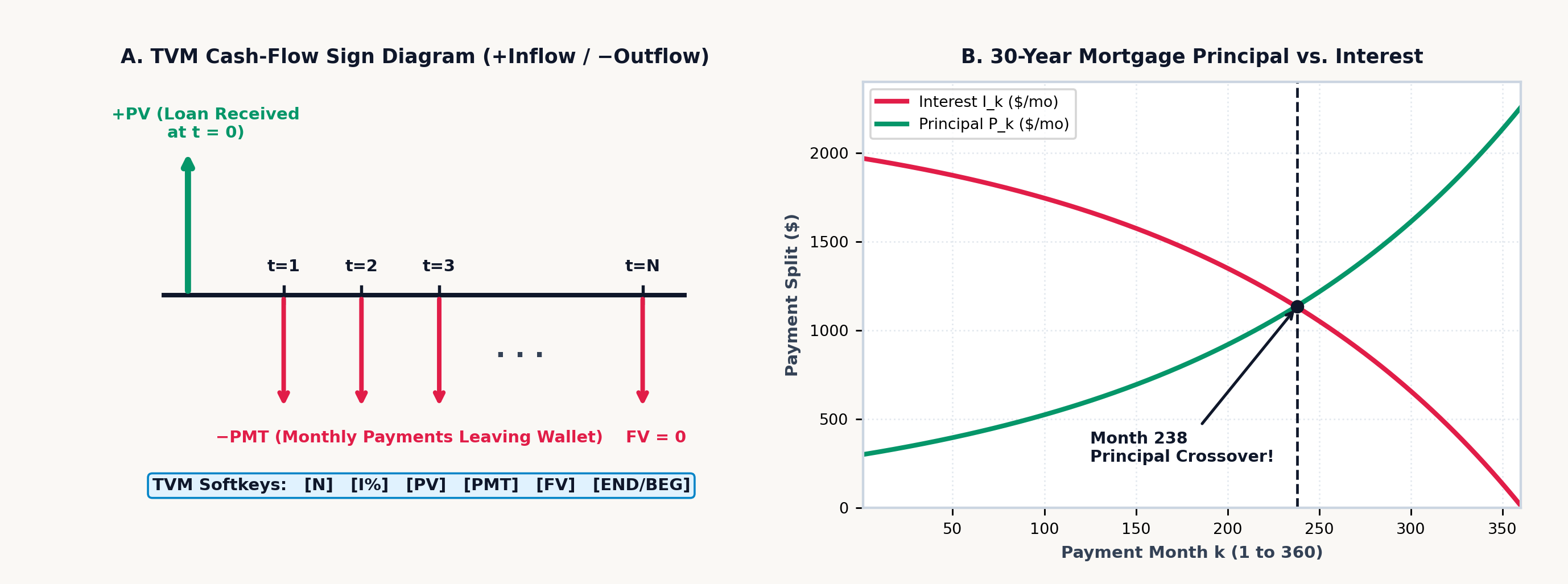
The three terms on the left-hand side of the Five-Variable TVM Balance Equation sum to zero (Figure 11.1). That algebraic zero enforces Cash-Flow Sign Conservation: money has a physical direction relative to your pocket. Cash inflows (\(+\), money received at loan closing, bond coupons collected, or maturity redemptions withdrawn) carry a positive sign; cash outflows (\(-\), monthly payments sent to a lender, purchase price paid for a bond, or savings deposits contributed to a fund) carry a negative sign. If an investor enters both \(\text{PV}\) and \(\text{FV}\) as positive inflows with \(\text{PMT} = 0\), there is no real interest rate \(i > -1\) at which two positive cash flows sum to zero.
In the zero-interest limit (\(\lvert i\rvert < 10^{-14}\)), the indeterminacy \(\frac{(1 + i)^N - 1}{i} \to \frac{0}{0}\) resolves to its analytical L'Hôpital limit \(N\), and an unknown periodic rate \(i\) is isolated across \([-99.99\%, +1,000\%]\) by sweeping a \(240\)-interval sign-change bracket followed by \(100\) bisection refinements. Commercial accounting also distinguishes between continuous compounding precision and printed ledger precision: if a wholesale unit price of \(\$85\) plus \(8.25\%\) tax equals \(\approx \$92.013\) internally ($92.01 when displayed to two decimal places), multiplying the unrounded internal figure across \(1,000\) units yields \(\$92,012.50\), while multiplying the printed unit invoice of \(\$92.01\) by \(1,000\) yields \(\$92,010\)—a \(\$2.50\) ledger discrepancy unless the unit line item is rounded to display precision before extending the invoice.
Behind the five-variable balance equation sit four classical actuarial identities—ordinary annuities, loan amortization, sinking funds, and perpetuities—that govern corporate debt, municipal infrastructure finance, and lifecycle pension planning over a schedule of \(n = N\) compounding periods at periodic rate \(i\):
The bracketed annuity present-value factor \(a_{\overline{n}|i} = \frac{1 - (1+i)^{-n}}{i} = \frac{1}{i} - \frac{(1+i)^{-n}}{i}\) has a clean intuitive decomposition: it is the difference between a perpetuity starting today (worth \(\frac{1}{i}\) per dollar of payment) and an identical perpetuity deferred \(n\) periods into the future (worth \(\frac{(1+i)^{-n}}{i}\) today), which cancels every payment after period \(n\) and leaves only the first \(n\) payments. Multiplying that present-value factor by \((1 + i)^n\) shifts the valuation to horizon \(t = n\), giving the future-value accumulation factor \(s_{\overline{n}|i} = \frac{(1+i)^n - 1}{i}\), where the numerator \((1+i)^n - 1\) is the net compound interest earned by a single dollar over \(n\) periods. Taking the reciprocals of those two factors yields the Capital-Recovery Identity \(\frac{i}{1 - (1+i)^{-n}} = \frac{i}{(1+i)^n - 1} + i\), which states that amortizing a \(\$1\) loan over \(n\) periods (left side) is financially identical to paying periodic interest \(i\) on the whole dollar while depositing \(\frac{i}{(1+i)^n - 1}\) each period into a sinking fund earning rate \(i\) to retire the \(\$1\) principal at maturity \(t = n\).
Discounting \(n = 48\) monthly lease payments of \(PMT = \$400\) at \(i = 0.65\%\) per month (\(7.8\%\) APR \(\div 12\)) gives \((1 + i)^{-48} \approx 0.733\), an annuity factor of \(a_{\overline{48}|i} \approx 41.12\), and a present value of \(PV \approx \mathbf{\$16,447.94}\); depositing \(PMT = \$500\) monthly for \(n = 32\text{ months}\) at \(i = 0.75\%\) per month (\(9\%\) APR \(\div 12\)) gives \(s_{\overline{32}|i} \approx 36.015\) and accumulates to \(FV \approx \mathbf{\$18,007.41}\). Similarly, amortizing an equipment loan of \(PV = \$28,000\) over \(n = 60\text{ months}\) at \(i = 0.75\%\) per month (\(9\%\) APR \(\div 12\)) requires a monthly payment of \(PMT \approx \mathbf{\$581.23}\), while accumulating a target replacement fund of \(FV = \$22,000\) over \(n = 60\text{ months}\) at \(i = 0.6\%\) per month (\(7.2\%\) APR \(\div 12\)) requires a monthly sinking-fund deposit of \(PMT_{\text{sink}} \approx \mathbf{\$305.71}\).
When an annuity has no maturity date at all (\(n \to \infty\)) and pays a fixed periodic cash flow \(PMT\) in perpetuity, the deferred-perpetuity tail \((1 + i)^{-n}\) vanishes as \(n \to \infty\), leaving the present value of a flat perpetuity \(PV_{\text{flat}}\). More generally, in the Gordon Growth Dividend Discount Model, if an university endowment payout or corporate dividend starts at \(D_1\) one period from today and grows perpetually at a constant periodic rate \(g\) while discounted at required return \(r > g\), the infinite geometric series converges to \(PV_{\text{growing}}\):
Both perpetuity denominators reflect a simple self-sustaining fund balance. A principal endowment of \(PV_{\text{flat}} = PMT / i\) invested at rate \(i\) generates \(PV_{\text{flat}} \times i = PMT\) of interest every period forever without ever touching the principal. When the payout must instead grow by a fraction \(g\) each period, the fund cannot distribute its entire return \(r\): the first \(g\) of the return \(r\) must be plowed back into the principal so the endowment base itself grows by \(g\) each period, leaving only the net return spread \((r - g)\) in the denominator of \(PV_{\text{growing}} = \frac{D_1}{r - g}\) available to fund the current payout \(D_1\). An endowment chair or preferred share paying a flat annual distribution of \(PMT = \$1,200\) forever discounted at \(i = 6\%\) (\(0.06\)) has a present value of \(PV_{\text{flat}} = \$1,200 / 0.06 = \mathbf{\$20,000}\); if that \(\$1,200\) initial distribution grows by \(g = 2\%\) per year forever to offset inflation (\(r - g = 0.04\)), its present value jumps by \(50\%\) to \(PV_{\text{growing}} = \$1,200 / (0.06 - 0.02) = \mathbf{\$30,000}\).
11.2 Bond Immunization, Macaulay Duration & Capital Budgeting
Beyond individual mortgages and savings plans, institutional fixed-income management and corporate capital budgeting extend discounting to multi-year bond cash flows, interest-rate immunization, and uneven project streams.
11.2.1 The Term Structure of Interest Rates, Bond Immunization & Macaulay Duration
A fixed-rate government or corporate bond is a pure five-variable TVM contract: the issuer promises to pay a periodic coupon cash flow \(C\) every period for \(N\) periods (PMT \(= C\)) and to return the face or par value \(M\) (conventionally \(M = \$100\) or \(\$1,000\)) at maturity \(t = N\) (FV \(= M\)). When the market prices the bond at an annualized Yield to Maturity (YTM) \(y\) compounded \(m\) times per year—quoted on Wall Street on a semi-annual Bond-Equivalent Yield (BEY, \(m = 2\)) basis where each period discounts at \(i = y / m\)—the investor pays the bond purchase price \(P\) today (PV \(= -P\), negative because cash leaves the buyer's hands):
The bond price \(P\) is the sum of two present-value components: the first term discounts the \(N\)-period stream of level coupons \(C\) using the ordinary annuity factor at periodic yield \(y/m\), and the second term discounts the single maturity par redemption \(M\) across all \(N\) periods by \((1 + y/m)^{-N}\). When the market yield equals the stated annual coupon rate \(c = mC/M\) (\(y = c\)), the bond trades at par (\(P = M\)); when market interest rates rise above the coupon rate (\(y > c\)), the bond trades at a discount below par (\(P < M\)) so the capital gain \((M - P)\) at maturity supplements the coupon; and when market rates fall below the coupon rate (\(y < c\)), the bond trades at a premium above par (\(P > M\)).
When a bond settles \(d_{\text{elapsed}}\) days into a \(d_{\text{period}}\)-day coupon period, the buyer pays the Dirty (Invoice) Price \(P_{\text{dirty}} = P_{\text{clean}} + C(d_{\text{elapsed}} / d_{\text{period}})\), which adds the seller's prorated accrued interest \(AI\) to the quoted Clean Price \(P_{\text{clean}}\). Trading screens quote clean prices because \(P_{\text{dirty}}\) rises in a daily sawtooth pattern as each coupon date approaches and drops by \(C\) on the ex-coupon date, whereas \(P_{\text{clean}}\) moves only when market yields or credit spreads change. On a \(\$1,000\) par corporate bond with a \(6\%\) semi-annual coupon (\(C = \$30\) every \(180\text{ days}\)) quoted at \(P_{\text{clean}} = \$984.50\) and settling \(45\text{ days}\) into a \(180\text{-day}\) period, accrued interest is \(AI = \$30 \times (45 / 180) = \$7.50\), yielding an invoice settlement price of \(P_{\text{dirty}} = \mathbf{\$992}\). At a semi-annual quote of \(y_{\text{BEY}} = 6.8\%\) (\(i_{\text{semi}} = 3.4\%\)), compounding across two half-years yields an Effective Annual Yield of \(\text{EAY} = (1.034)^2 - 1 \approx \mathbf{6.916\%}\).
If a portfolio manager holds a 10-year zero-coupon bond (which pays nothing until Year 10) alongside a 10-year \(8\%\) coupon bond (which returns a substantial portion of its cash flows in Years 1 through 9), both instruments share the same 10-year calendar maturity, yet the zero-coupon bond is far more sensitive to interest-rate shocks. Modeling a bond as a physical beam along the time axis \(t = 1, 2, \dots, N\)—where each period \(t\) delivers a total cash flow \(C_t\) (\(C_t = C\) prior to maturity and \(C_N = C + M\) at maturity) whose present value \(PV(C_t) = C_t (1 + y/m)^{-t}\) acts as a downward gravitational weight—locates the center of mass (fulcrum) of those present-value weights at the Macaulay Duration \(D_{\text{mac}}\) (in periods), its annualized counterpart \(D_{\text{yr}}\) (in years), and the yield-slope Modified Duration \(D^*\):
Each payment time \(t\) in \(D_{\text{mac}}\) is weighted by the fraction \(\frac{C_t(1+y/m)^{-t}}{P}\) of the bond's total price \(P\) recovered at that period, and dividing \(D_{\text{mac}}\) by \(m\) periods per year converts that balance point into calendar years \(D_{\text{yr}}\). Differentiating \(P(y)\) with respect to the annualized yield \(y\) pulls down a factor of \(-(1 + y/m)^{-1}\) from the chain rule, proving that Modified Duration \(D^* = D_{\text{yr}} / (1 + y/m)\) measures the exact first-order fractional price change \(\Delta P / P \approx -D^* \Delta y\) for a small yield shift \(\Delta y\), while Dollar Duration (DV01) \(= P \cdot D^* \times 10^{-4}\) gives the dollar price change per \(1\text{ basis point}\) (\(0.01\%\)) yield move.
Because the discount factor \((1 + y/m)^{-t}\) is convex (bowing upward as yields fall and flattening out as yields rise), the linear tangent approximation \(-D^*\,\Delta y\) overstates price losses when yields jump and understates price gains when yields fall. Differentiating \(P(y)\) a second time with respect to yield \(y\) defines Bond Convexity (\(\text{Conv}\), in \(\text{years}^2\)) and the second-order Taylor quadratic for the fractional price change \(\Delta P / P\) under a yield shift \(\Delta y\):
The linear term \(-D^*\,\Delta y\) traces the tangent-line price drop when yields rise (\(\Delta y > 0\)), while the quadratic term \(+\frac{1}{2}\,\text{Conv}\,(\Delta y)^2\) captures the upward parabolic bow of the price-yield curve. Because \((\Delta y)^2\) is positive whether interest rates rise (\(\Delta y > 0\)) or fall (\(\Delta y < 0\)), positive convexity always works in the bondholder's favor—cushioning price declines when rates spike and amplifying capital gains when rates drop.
On a 3-year annual-pay (\(m = 1\)) corporate bond with a \(6\%\) coupon (\(C_1 = 6,\; C_2 = 6,\; C_3 = 106\)) trading at par (\(P = 100\) at yield \(y = 0.06\)), discounting the time-weighted cash flows (\(1\times 6 = 6\), \(2\times 6 = 12\), and \(3\times 106 = 318\)) by stepping backward from Year 3 to Year 1 and dividing by \(1.06\) at each year—\(\frac{1}{1.06}(6 + \frac{1}{1.06}(12 + \frac{318}{1.06})) \approx 283.339\)—and dividing by \(P = 100\) gives Macaulay Duration \(D_{\text{yr}} \approx \mathbf{2.833\text{ years}}\) and Modified Duration \(D^* \approx 2.833 / 1.06 \approx \mathbf{2.673\text{ years}}\) (\(\text{DV01} \approx 2.673\text{ cents}\) per \(\$100\) par). Summing the second-moment convexity terms \(\sum_{t=1}^3 \frac{t(t+1)C_t}{(1+y)^t} = \frac{2(6)}{1.06} + \frac{6(6)}{1.06^2} + \frac{12(106)}{1.06^3} \approx 1,111.356\) and dividing by \(100 \times (1.06)^2 = 112.36\) yields Convexity \(\text{Conv} \approx \mathbf{9.891\text{ yr}^2}\); under a \(+200\text{ bps}\) (\(\Delta y = +0.02\)) rate shock, linear duration predicts \(-2.673 \times 0.02 = -5.346\%\), while adding the convexity cushion \(+\frac{1}{2}(9.891)(0.02)^2 \approx +0.198\%\) predicts \(\Delta P / P \approx \mathbf{-5.148\%}\) (matching the exact repriced bond loss \(\approx -5.154\%\) to within six-thousandths of a percent).
Macaulay Duration carries physical units of years because it marks the balance point between two opposing interest-rate risks. When interest rates rise (\(\Delta y > 0\)), a bondholder experiences two opposing forces: the bond's immediate market price falls (Price Risk), while all future coupon payments can be reinvested at the higher interest rate (Reinvestment Risk). At the investment horizon equal to the bond's Macaulay Duration (\(H = D_{\text{yr}}\)), the first-order price loss and cumulative coupon reinvestment gain cancel to zero. To immunize a liability due at target horizon \(H\) using two bonds of durations \(D_1 < H < D_2\), a portfolio manager chooses portfolio weights \(w_1\) and \(w_2 = 1 - w_1\) so the value-weighted portfolio duration matches the horizon (\(w_1 D_1 + (1 - w_1)D_2 = H\)), solving for \(w_1 = \frac{D_2 - H}{D_2 - D_1}\), which divides the long bond's excess duration \((D_2 - H)\) by the total duration span \((D_2 - D_1)\) between the two bonds.
Consequently, a pension fund facing a fixed \(\$10,000,000\) liability due at horizon \(H = 5\text{ years}\) immunizes its balance sheet against parallel interest-rate shifts by blending a 2-year Treasury note (\(D_1 = 1.94\text{ years}\)) and a 10-year Treasury bond (\(D_2 = 7.8\text{ years}\)) with weights \(w_1 = \frac{D_2 - H}{D_2 - D_1} = \frac{7.8 - 5}{7.8 - 1.94} \approx \mathbf{47.782\%}\) (\(\approx \$4,778,157\)) and \(w_2 = 1 - w_1 \approx \mathbf{52.218\%}\) (\(\approx \$5,221,843\)) so the asset portfolio's duration matches \(H = 5\text{ years}\) while its convexity exceeds the liability's convexity.
11.2.2 Capital Budgeting, Reverse-Time Horner Discounting & Corporate Hurdle Rates
The five-variable TVM balance equation assumes a level periodic cash flow \(\text{PMT}\), yet corporate capital projects, manufacturing plants, and venture startups generate uneven cash flows \(C_0, C_1, C_2, \dots, C_T\) across time—typically an initial capital expenditure \(C_0 < 0\) at \(t = 0\) followed by variable operating inflows \(C_t\) as production scales up.
Rather than raising \((1 + r)\) to \(T\) separate powers, we can write Net Present Value (NPV) discounted at periodic cost of capital \(r\) as a polynomial in the single-period discount factor \(u = (1 + r)^{-1}\). Applying reverse-time Horner nesting then evaluates an arbitrary \(T\)-period uneven NPV by nested division from the final horizon \(t = T\) backward to \(t = 0\):
Working outward from the innermost terminal cash flow \(C_T\), a single division by \((1 + r)\) discounts \(C_T\) back to period \(T - 1\) where it adds directly to \(C_{T-1}\); each subsequent division by \((1 + r)\) steps the running subtotal one period closer to the present day until the entire stream reaches \(t = 0\) to combine with the upfront outlay \(C_0\). In a capital manufacturing line requiring an initial investment of \(C_0 = -\$50,000\) at \(t = 0\) and generating uneven net operating inflows of \(C_1 = +\$12,000\), \(C_2 = +\$18,000\), \(C_3 = +\$22,000\), and \(C_4 = +\$25,000\) over Years 1 through 4 at a corporate hurdle rate of \(r = 10\%\) (\(1 + r = 1.1\)), stepping backward from Year 4 (\(25,000 / 1.1 + 22,000 \approx 44,727.27 \to \div 1.1 + 18,000 \approx 58,661.16 \to \div 1.1 + 12,000 \approx 65,328.32 \to \div 1.1 \approx \$59,389.39\) present value of inflows) and subtracting the \(\$50,000\) initial outlay yields \(\text{NPV}(10\%) \approx \mathbf{+\$9,389.39}\) and a Profitability Index of \(\text{PI} = \text{PV}_{\text{inflows}} / |C_0| \approx 59,389.39 / 50,000 \approx \mathbf{1.188}\).
The zero crossing \(\text{NPV}(r^*) = 0\) defines the Internal Rate of Return (IRR)—the break-even discount rate at which the present value of future inflows equals \(|C_0|\) (for the 4-year manufacturing line, locating the root of the Horner polynomial gives \(1 + r^* \approx 1.174\), or \(\text{IRR} \approx \mathbf{17.434\%}\), which exceeds a \(10\%\) hurdle rate by more than \(740\text{ basis points}\)). Because \(\text{NPV}(r) = 0\) is a \(T\)-th degree polynomial in \(u = (1 + r)^{-1}\), Descartes's rule of signs guarantees a unique positive root \(r^*\) when the cash-flow sequence changes sign exactly once (\(C_0 < 0\) followed by \(C_1, \dots, C_T \ge 0\)). If a project requires a large environmental remediation outflow at the end of its life (\(C_0 < 0,\; C_1 > 0,\; C_2 < 0\), changing sign twice), \(\text{NPV}(r)\) can cross zero at two distinct positive IRRs.
Standard IRR implicitly assumes that every intermediate cash inflow \(C_t\) is reinvested at the project's own high IRR \(r^*\); Modified Internal Rate of Return (MIRR) resolves multiple roots and applies a realistic reinvestment rate \(r_{\text{reinv}}\) by compounding positive inflows forward to horizon \(T\) as \(\text{TV} = \sum_{C_t > 0} C_t (1 + r_{\text{reinv}})^{T-t}\), discounting negative outflows to \(t = 0\) at financing rate \(r_{\text{fin}}\) as \(\text{PV}_{\text{out}} = \sum_{C_t < 0} |C_t|(1 + r_{\text{fin}})^{-t}\), and taking the \(T\)-th root: \(\text{MIRR} = (\text{TV} / \text{PV}_{\text{out}})^{1/T} - 1\). For a 3-year project with \(C_0 = -\$1,000\), inflows \(C_1 = \$400,\; C_2 = \$500,\; C_3 = \$600\), and corporate reinvestment rate \(r_{\text{reinv}} = 10\%\), standard IRR is \(\approx 21.65\%\), while compounding the inflows to Year 3 at \(10\%\) gives \(\text{TV} = 400(1.1)^2 + 500(1.1) + 600 = \$1,634\) and a realistic \(\text{MIRR} = (1634 / 1000)^{1/3} - 1 \approx \mathbf{17.783\%}\).
When comparing two industrial machines with unequal service lives \(N\)—such as a carbon-steel chemical pump lasting \(N_A = 4\text{ years}\) (upfront capital outlay \(C_{0,A} = \$24,000\), annual maintenance \(C_{\text{maint},A} = \$4,500/\text{yr}\)) versus a corrosion-resistant titanium pump lasting \(N_B = 8\text{ years}\) (\(C_{0,B} = \$42,000\), annual maintenance \(C_{\text{maint},B} = \$2,200/\text{yr}\)) at cost of capital \(r = 8\%\)—a raw present-value comparison is invalid because the 4-year pump must be replaced twice as often. Dividing each machine's upfront purchase price \(C_0\) by its \(N\)-year annuity factor \(a_{\overline{N}|r} = \frac{1 - (1+r)^{-N}}{r}\) converts the lump-sum price into an equivalent annual capital rent, and adding the annual operating maintenance \(C_{\text{maint}}\) defines the Equivalent Annual Cost (EAC \(= \frac{C_0}{a_{\overline{N}|r}} + C_{\text{maint}}\)): Machine A costs \(\text{EAC}_A \approx \$7,246.10 + \$4,500 \approx \mathbf{\$11,746.10/\text{yr}}\), while Machine B costs \(\text{EAC}_B \approx \$7,308.62 + \$2,200 \approx \mathbf{\$9,508.62/\text{yr}}\), saving \(\approx \$2,237.48\) every year.
At the enterprise level, management evaluates how effectively shareholders' capital generates profit via Return on Equity (\(\text{ROE} = \text{Net Income} / \text{Equity}\)) and sets the firm-wide project hurdle rate using its capital structure—the market value of equity \(E\), market value of debt \(D\), total firm value \(V = E + D\), required return on equity \(r_e\), pre-tax cost of debt \(r_d\), and corporate tax rate \(\tau_c\)—through the DuPont Three-Factor ROE Identity and the Weighted Average Cost of Capital (WACC):
Algebraically, \(\text{Revenue}\) and \(\text{Assets}\) cancel across the three DuPont ratios to recover \(\text{Net Income} / \text{Equity}\), decomposing shareholder return into three operational levers: how much profit each sales dollar keeps (Net Profit Margin), how rapidly the asset base generates sales (Asset Turnover), and how much debt amplifies equity (Equity Multiplier). Meanwhile, \(\text{WACC}\) weights the cost of equity \(r_e\) and pre-tax cost of debt \(r_d\) by their capital-structure shares \(E/V\) and \(D/V\), multiplying the debt term by \((1 - \tau_c)\) because corporate interest payments are tax-deductible—a tax shield in which the government absorbs fraction \(\tau_c\) of every interest dollar paid. In a manufacturer with Net Income \(\$18\text{M}\), Revenue \(\$150\text{M}\) (\(\text{Margin} = 12\%\)), Total Assets \(\$120\text{M}\) (\(\text{Turnover} = 1.25\times\)), and Shareholders' Equity \(\$60\text{M}\) (\(\text{Leverage} = 2\times\), Debt \(D = \$60\text{M}\), so \(E/V = D/V = 0.5\)), with cost of equity \(r_e = 11.5\%\), pre-tax debt cost \(r_d = 6\%\), and corporate tax rate \(\tau_c = 25\%\), the three DuPont levers multiply to \(\text{ROE} = 0.12 \times 1.25 \times 2 = \mathbf{30\%}\) against a corporate hurdle rate of \(\text{WACC} = 0.5(11.5\%) + 0.5(6\%)(0.75) = \mathbf{8\%}\) (generating a \(+22\%\) Economic Value Added spread).
11.3 Financial Synthesis on the Stack: From Mortgages to Option Pricing
On the SC-32, two dedicated financial interfaces map percentage scaling and five-variable cash-flow discounting onto the four-register stack:
- Base-Preserving Percentage Operators (
[↱] [%]and[↱] [%CHG]) & Ledger Rounding ([↰] [RND]): If you compute \(20\%\) of \(\$85\) on an ordinary algebraic calculator by multiplying \(85 \times 0.2 = 17\), the binary multiplication consumes both operands and overwrites the display with \(17\), discarding the original \(\$85\) base value just when you need to add or subtract that \(\$17\) tax, tip, or markdown. The SC-32's right-shifted percentage operations—[↱] [%]on[COS]and[↱] [%CHG]on[TAN]—preserve the base value in Register \(Y\) (while[↰] [RND], left-shifted on[RCL], rounds Register \(X\)'s internal 53-bit value to the activeFIX 2cent display whenever an invoice line item must be quantized to exact cents before multiplying by quantity):
| Operation | Mathematical Formula | Stack Before (Y, X) |
Stack After (Y, X) |
Subsequent Action (+ or -) |
|---|---|---|---|---|
Percentage ([↱] [%]) |
\(X' = Y \times \frac{X}{100}\) | Y = Base, X = Rate % |
Y = Base, X = Portion |
Addition adds tax/markup; subtraction deducts discount |
Percent Change ([↱] [%CHG]) |
\(X' = \frac{X - Y}{Y} \times 100\) | Y = Old, X = New |
Y = Old, X = Δ% |
Base preserved in Y for elasticity comparisons |
- The Five-Variable
[↰] [TVM]Softkey Workspace: Invoking[↰] [TVM]([x∥y]) opens the financial workspace and assigns the six top-row softkeys to:
All five financial registers (N for total periods, I% for periodic interest rate, PV for present value, PMT for periodic payment, and FV for future value) default to 0 (and can be reset to 0 at any time via CLEAR \(\to\) [CLVARS] or [CLREGS]), while the sixth softkey toggles between end-of-period ordinary annuities (END, the default) and beginning-of-period annuities due (BEG). Just like POLY for polynomial coefficients, the TVM softkey bar lets you enter values directly on the softkeys without pressing STO or RCL, and solves directly on the target variable softkey without pressing XEQ: any intervening non-TVM keystroke (such as typing a digit, changing sign, or executing an arithmetic operator) arms the next financial softkey to store Register \(X\) into that slot (STO N, STO I%, etc.), whereas tapping another financial softkey immediately afterward solves the master balance equation for that unknown variable and places the result in Register \(X\). Because unentered slots default to 0, a pure lump-sum compounding problem with no periodic payments leaves PMT untouched at 0, and a fully amortizing mortgage with zero terminal balance leaves FV untouched at 0.
11.3.1 Base-Preserving Percentages, Elasticity & Gross-Margin Pricing
When a software-as-a-service (SaaS) platform raises its monthly subscription price from \(\$40\) to \(\$46\) while active seat count shifts from \(1,250\) to \(1,150\), evaluating percent change on price (\(+15\%\) in \(X\), with \(\$40\) preserved in \(Y\)) and then on seat volume (\(-8\%\) in \(X\), lifting \(+15\%\) into \(Z\) while preserving \(1,250\) in \(Y\)) leaves \(-8\%\) in \(X\) and \(+15\%\) in \(Z\); rolling or swapping past the preserved \(1,250\) base to divide \(\% \Delta Q = -8\%\) by \(\% \Delta P = +15\%\) yields a price elasticity of demand \(E_d \approx \mathbf{-0.533}\) (confirming inelastic demand since \(|E_d| < 1\), so monthly revenue rises from \(\$50,000\) to \(\$52,900\)).
Because the percentage operator leaves the original base untouched in Register \(Y\) while placing the computed dollar portion \(Y \times (X / 100)\) in Register \(X\), adding an \(8.25\%\) sales tax to an \(\$85\) invoice computes the \(\approx \$7.013\) tax portion in \(X\) and adds it to \(\$85\) in \(Y\) for a gross invoice of \(\$92.01\) (\(\approx 92.013\) internally, which rounding to display precision under FIX 2 quantizes to exact $92.01 so hidden fractional cents never accumulate across bulk invoice lines). Deducting a \(15\%\) OEM contract discount from a \(\$1,200\) optical sensor module places the \(\$180\) discount in \(X\) and subtracts it from \(\$1,200\) in \(Y\) to yield \(\$1,020\); and adding an \(18\%\) customs tariff and freight surcharge (\(\$2,565\)) to a \(\$14,250\) laboratory instrument shipment before dividing by \(4\) splits the \(\$16,815\) landed cost into \(\$4,203.75\) per department.
11.3.2 Lifecycle Wealth Accumulation & Two-Stage Retirement Chaining
Future-value accumulation and present-value amortization chain across a two-stage retirement plan: an engineer saves \(\text{PMT}_{\text{save}} = -\$1,000\) per month for \(30\text{ years}\) (\(N_1 = 360\text{ months}\)) during her working career in an equity index portfolio earning \(7.2\%\) APR (\(i_1 = 0.6\%\) per month), and then transitions at retirement into a conservative bond/income portfolio earning \(4.8\%\) APR (\(i_2 = 0.4\%\) per month) from which she withdraws a level monthly pension over a \(25\text{-year}\) retirement horizon (\(N_2 = 300\text{ months}\), exhausting the nest egg to \(FV_2 = 0\)).
In Stage 1 (END mode), storing \(N_1 = 360\), \(I\% = 0.6\), \(PV_1 = 0\), and \(\text{PMT}_1 = -1,000\) in the TVM workspace and solving for future value accumulates a 30-year retirement nest egg of \(FV_1 \approx \mathbf{\$1,269,225.44}\) (making each deposit on the first day of the month in BEG mode multiplies that nest egg by \(1.006\) to \(\approx \$1,276,840.79\)—an extra \(\$7,615.35\) of compound growth just from shifting deposits 30 days earlier). Negating that Stage 1 nest egg into Stage 2 opening capital (\(PV_2 \approx -\$1,269,225.44\)), setting \(FV_2 = 0\), \(N_2 = 300\text{ months}\), and \(I\% = 0.4\), and solving for periodic payment funds a sustainable retirement income of \(\text{PMT}_2 \approx \mathbf{+\$7,272.62\text{ per month}}\) for 25 years.
11.3.3 Mortgage Amortization Crossover, Balloon Notes & Curtailment
When a homebuyer finances a \(PV = +\$400,000\) 30-year fixed-rate mortgage (\(N = 30 \times 12 = 360\) months) at a nominal APR of \(6.5\%\) compounded monthly (\(I\% = 6.5 / 12 \approx 0.542\%\) per month) with full amortization (\(FV = 0\)), storing the four known parameters in the TVM workspace and solving for periodic payment yields the level monthly outflow \(\text{PMT} \approx \mathbf{-\$2,528.27}\) (\(\approx -2,528.272\) in FIX 3, negative because cash flows out to the lender). Figure 11.2 illustrates the same \(\$400,000\), \(360\text{-month}\) mortgage at \(6\%\) APR (\(I\% = 0.5\%\)), where \(\text{PMT} \approx -\$2,398.202/\text{month}\).
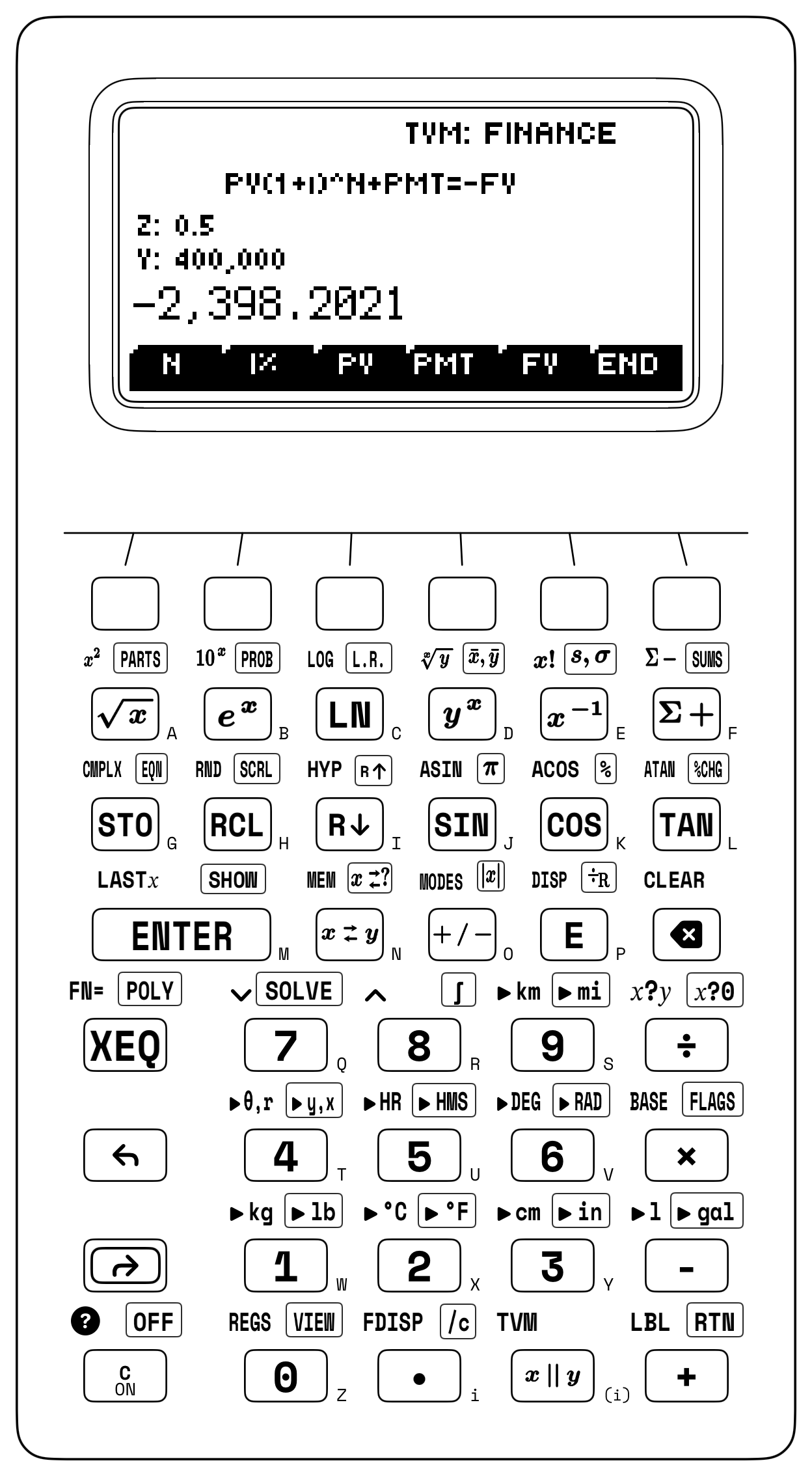
The internal split of that \(\$2,528.27\) monthly payment explains why early mortgage payments barely dent the principal. In Month 1, the borrower owes one month's periodic interest \(i = 0.065 / 12\) on the entire \(\$400,000\) opening balance: \(\text{Interest}_1 = \$400,000 \times (0.065/12) \approx \mathbf{\$2,166.67}\), leaving only \(\text{Principal}_1 \approx \$2,528.27 - \$2,166.67 \approx \mathbf{\$361.61}\) to reduce the debt. More than \(85.7\%\) of the first mortgage check pays interest, leaving a Month 1 ending balance of \(\approx \$399,638.39\). Over all \(360\) months, total cash paid is \(360 \times |\text{PMT}| \approx \$910,177.97\), meaning cumulative interest paid over 30 years is \(\approx \mathbf{\$510,177.97}\)—more than \(1.275\times\) the original price of the home.
Because the principal portion of payment \(t\) is simply the final payment \(|\text{PMT}|\) discounted backward across the remaining \((N - t + 1)\) months as \(\text{Principal}_t = |\text{PMT}|(1 + i)^{-(N - t + 1)}\), the Amortization Crossover Month \(t_{\text{cross}}\)—the first month in which more than half of your monthly payment reduces principal—occurs when \((1 + i)^{-(N - t_{\text{cross}} + 1)} > \frac{1}{2}\):
The inequality states that the number of payments remaining on the mortgage \((N - t_{\text{cross}} + 1)\) must fall inside one compound-interest doubling time \(\frac{\ln 2}{\ln(1+i)} \approx 128.31\text{ months}\) (\(\approx 10.7\text{ years}\)) prior to maturity; subtracting the integer part \(\lfloor 128.31 \rfloor = 128\) from \(360 + 1\) locates the exact crossover at Month 233. Since the TVM workspace retains all stored parameters across solves, updating \(N\) to \(84\) and querying future value shows that if the homeowner sells or refinances after 7 years (\(84\text{ months}\)), the remaining payoff balance is \(FV \approx \mathbf{-\$361,664.98}\), so out of \(\approx \$212,374.86\) in total cash outflows (\(84 \times \$2,528.27\)), principal has fallen by only \(\approx \$38,335.02\) while \(\approx \$174,039.84\) was consumed by interest.
An intermediate future-value query also prices commercial real-estate balloon notes: when a \(\$1,500,000\) property amortizes over a 25-year schedule (\(N = 300\text{ months}\)) at \(7.2\%\) APR (\(I\% = 0.6\%/\text{month}\), \(\text{PMT} \approx \mathbf{-\$10,793.83/\text{month}}\)) with a mandatory 5-year balloon maturity, updating \(N\) to \(60\) and querying future value reveals the Year 5 refinancing balloon balance of \(FV \approx \mathbf{-\$1,370,907.47}\). If the residential borrower instead adds an extra \(\$300\) per month toward principal (increasing the monthly outflow to \(\text{PMT} \approx -\$2,828.27\) and resetting \(FV = 0\) after any intermediate balance query), solving for \(N\) slashes the mortgage payoff horizon from \(360\text{ months}\) down to \(\approx \mathbf{268.93\text{ months}}\) (\(\approx 22.4\text{ years}\)), eliminating \(\approx 91.07\text{ months}\) (\(\approx 7.6\text{ years}\)) of debt service and saving \(\approx \mathbf{\$149,581.85}\) in cumulative interest.
11.3.4 Fixed-Income Valuation: Corporate Bond YTM, Duration & Convexity
When a 10-year corporate bond (\(N = 20\) semi-annual periods, par \(FV = \$1,000\), \(5.5\%\) annual coupon paid as \(\text{PMT} = \$27.50\) every six months) trades in the secondary market at a discount price of \(PV = -\$942.50\), storing the four cash-flow terms in the TVM workspace and solving for the periodic rate yields the semi-annual yield \(i_{\text{semi}} \approx \mathbf{3.142\%}\), which doubles to a Wall Street Bond-Equivalent Yield of \(\text{BEY} \approx \mathbf{6.283\%}\).
The two-period factor \((1 + i_{\text{semi}})^2 - 1\) converts that nominal semi-annual quote into an Effective Annual Yield of \(\text{EAY} \approx \mathbf{6.382\%}\), while inverting the solve (entering a target yield \(I\% = y_{\text{BEY}} / 2\) and querying present value) prices any fixed-coupon bond at par, discount, or premium. And when cash flows vary from period to period, as in uneven project NPV and multi-year bond duration and convexity, stepping backward from maturity via Horner division by \((1 + r)\) accumulates the discounted stream in Register \(X\).
11.3.5 Portfolio Risk-Adjusted Returns, Kelly Sizing & Black–Scholes Option Pricing
Quantitative asset management extends discounting and compounding to uncertain risky cash flows through three models: the Capital Asset Pricing Model (CAPM) and Sharpe Ratio, the Kelly Capital Growth Criterion, and Black–Scholes–Merton Option Pricing.
Across a diversified mean-variance portfolio, firm-specific idiosyncratic variance cancels out, leaving only systematic market beta \(\beta_i = \frac{\operatorname{Cov}(R_i, R_m)}{\operatorname{Var}(R_m)} = r_{im}\frac{\sigma_i}{\sigma_m}\), which multiplies the correlation coefficient \(r_{im}\) between asset \(i\) and the market by the ratio of asset return volatility \(\sigma_i\) to market return volatility \(\sigma_m\) (identical to the least-squares regression slope \(m\) when asset returns \(R_i\) in \(Y\) are regressed against market returns \(R_m\) in \(X\)). Given the risk-free Treasury rate \(R_f\), expected market return \(R_m\), portfolio return \(R_p\) with total portfolio volatility \(\sigma_p\), and individual asset or fund return \(R_i\), three complementary metrics along the Security Market Line (SML) evaluate risk-adjusted performance:
Each metric isolates a specific dimension of risk and return: the Sharpe Ratio (\(S\)) divides excess portfolio return \((R_p - R_f)\) by total return volatility \(\sigma_p\) (scaling with the square root of time as \(S_{\text{ann}} = \sqrt{K}\,S_{\text{period}}\) across \(K = 252\) trading days or \(K = 12\) months per year); the Treynor Ratio (\(T_i\)) divides excess return \((R_i - R_f)\) by systematic market beta \(\beta_i\) to measure compensation per unit of non-diversifiable market risk; and Jensen's Alpha (\(\alpha_i\)) subtracts the passive CAPM benchmark return \([R_f + \beta_i(R_m - R_f)]\) from the actual return \(R_i\) to isolate active manager skill above passive market exposure. For a fund returning \(R_i = 21.8\%\) when the market returns \(R_m = 13.2\%\), the risk-free rate is \(R_f = 4.2\%\) (\(R_m - R_f = 9\%\)), and portfolio beta is \(\beta_i = 1.35\), the CAPM benchmark return is \(4.2\% + 1.35(9\%) = \mathbf{16.35\%}\), giving Jensen's Alpha \(\alpha_i = 21.8\% - 16.35\% = \mathbf{+5.45\%}\) (\(+545\text{ bps}\) of outperformance) and Treynor Ratio \(T_i = (21.8 - 4.2)/1.35 \approx \mathbf{13.037\%}\).
Once a strategy with a positive expected edge is identified, a risk manager must determine how much capital to allocate to each position. Maximizing the expected logarithmic compound growth rate \(G(f) = p\ln(1 + bf) + q\ln(1 - f)\) across a repeatable favorable wager (with win probability \(p\), loss probability \(q = 1 - p\), and net payoff odds \(b\)-to-\(1\)) yields the optimal Kelly fraction \(f^*\):
At the optimal fraction \(f^*\), the expected marginal log-utility of winning \(\frac{pb}{1 + bf^*}\) balances the expected marginal log-penalty of losing \(\frac{q}{1 - f^*}\); solving for \(f^* = \frac{pb - q}{b}\) divides the expected arithmetic edge per dollar risked \((pb - q)\) by the net payoff odds \(b\). Because betting more than \(2 f^*\) drives expected compound growth \(G(f)\) negative even when the wager has a positive arithmetic expectation, quantitative risk desks routinely allocate Half-Kelly (\(\frac{1}{2} f^*\)), capturing \(75\%\) of the maximum logarithmic growth rate while enduring only \(25\%\) of the variance.
The valuation of a European call option \(C\) and put option \(P\) with strike price \(K\) and time to expiration \(T\) (in years) on a non-dividend-paying underlying asset at spot price \(S_0\) with annualized return standard deviation (volatility) \(\sigma\) and continuously compounded risk-free rate \(r\) relies on dynamic replication. Because the underlying asset and the call option share the same geometric Brownian motion diffusion source, holding one call option against \(\Delta = \partial C / \partial S\) shorted shares cancels the stochastic diffusion term at every instant, forcing the hedged portfolio to grow deterministically at the risk-free rate \(r\).
This continuously rebalanced delta-hedged portfolio yields the closed-form Black–Scholes–Merton Formula and Put–Call Parity, pairing continuous exponential discounting \(K e^{-rT}\) with the standard normal cumulative distribution \(\Phi(z) = \frac{1}{\sqrt{2\pi}}\int_{-\infty}^z e^{-t^2/2}\,dt\):
Economically, the Black–Scholes call price \(C = S_0\Phi(d_1) - Ke^{-rT}\Phi(d_2)\) measures what you expect to receive minus what you expect to pay: \(S_0\Phi(d_1)\) is the delta-weighted present value of the underlying shares received if the call finishes in the money, and \(Ke^{-rT}\Phi(d_2)\) is the discounted strike price \(Ke^{-rT}\) multiplied by the risk-neutral exercise probability \(\Phi(d_2)\). Volatility enters \(d_1\) and \(d_2\) in two distinct ways: independent return variances add linearly over \(T\) periods so return dispersion grows with the square root of time (\(\sigma\sqrt{T}\)), whereas compounding log-normal price fluctuations bends upward exponentially, adding a continuous convexity drift of \(+\frac{1}{2}\sigma^2 T\) (Itô's correction) that separates the share-numeraire hedge ratio \(\Phi(d_1) = \Delta_{\text{call}}\) from the risk-neutral exercise probability \(\Phi(d_2)\) (\(S_T > K\)). Because holding a fiduciary call (\(C + K e^{-rT}\) invested in risk-free Treasury bills) produces the same terminal payoff \(\max(S_T, K)\) at expiration \(T\) as holding a protective put (\(S_0 + P\)), Put–Call Parity (\(P = C + K e^{-rT} - S_0\)) locks the European call and put prices together regardless of volatility \(\sigma\).
A single pass through the Sharpe Ratio (\(R_p = 18.4\%\), \(R_f = 4.2\%\), \(\sigma_p = 11.5\% \implies S \approx \mathbf{1.235}\)), Full- and Half-Kelly position sizing (\(p = 0.58\), \(q = 0.42\), \(b = 1.5 \implies f^* = \mathbf{30\%}\) and \(\frac{1}{2}f^* = \mathbf{15\%}\)), and Put–Call Parity (\(S_0 = \$105\), \(K = \$100\), \(r = 5\%\), \(T = 0.5\text{ yr}\), \(C = \$9.80 \implies K e^{-rT} \approx \$97.531\) and \(P \approx \mathbf{\$2.331}\)) lifts each completed metric up the four-register stack:
| Keystroke | Register T | Register Z | Register Y | Register X | What Happens on the Stack |
|---|---|---|---|---|---|
18.4 [ENTER] 4.2 [-] 11.5 [÷] |
\(0\) | \(0\) | \(0\) | \(1.235\) | Portfolio Sharpe Ratio \((18.4 - 4.2) / 11.5 \approx 1.235\) |
.58 [ENTER] 1 [ENTER] .58 [-] 1.5 [÷] |
\(1.235\) | \(1.235\) | \(0.58\) | \(0.28\) | Stage \(p = 0.58\) in \(Y\); evaluate loss-odds ratio \(q/b = 0.42/1.5 = 0.28\) in \(X\) |
[-] 2 [÷] |
\(1.235\) | \(1.235\) | \(1.235\) | \(0.15\) | Full Kelly \(f^* = 0.3 \to\) institutional Half-Kelly \(\frac{1}{2}f^* = 0.15\) (\(15\%\)) |
9.8 [ENTER] .05 [ENTER] .5 [×] [+/-] [eˣ] 100 [×] |
\(0.15\) | \(0.15\) | \(9.8\) | \(97.531\) | Stage call \(C = \$9.8\) in \(Y\); discounted strike \(K e^{-rT} \approx \$97.531\) in \(X\) |
[+] 105 [-] |
\(0.15\) | \(0.15\) | \(0.15\) | \(2.331\) | European Put \(P = C + Ke^{-rT} - S_0 \approx \$2.331\) (with \(\frac{1}{2}f^* = 0.15\) in \(Y, Z, T\)) |
11.3.6 Try It on the Stack
- Executive Gross-Margin Pricing vs. Markup: For a hardware product with unit cost \(C = \$60\) and target gross margin \(M = 40\%\) (\(0.4\)), evaluate the true gross-margin selling price \(P = C / (1 - M)\) and compare it against a \(40\%\) markup \(C(1 + 0.4)\). (Verified Register \(X\) results: gross-margin price \(\mathbf{\$100}\) vs. markup price \(\mathbf{\$84}\).)
- Mortgage Extra-Principal Payoff Acceleration: In the
TVMworkspace (withFVdefaulting to \(0\) inENDmode), store a \(PV = \$350,000\) loan at \(6.75\%\) APR (\(I\% = 6.75 / 12\%\) per month, entered as \(6.75 \div 12\)) with an accelerated monthly payment of \(\text{PMT} = -\$2,520.09\) (\(\approx \$250/\text{month}\) above the standard 30-year payment), and tap the first softkey to solve for the reduced payoff horizon \(N\). (Verified Register \(X\) result: \(N \approx \mathbf{270.928\text{ months}}\), cutting more than \(7.4\text{ years}\) off the 360-month mortgage.) - Single-Entry Kelly Optimal Allocation: Given win probability \(p = 0.62\) and net payoff odds \(b = 1.9\), evaluate the full Kelly percentage \(f^* = \left(p - \frac{1 - p}{b}\right) \times 100\%\) by subtracting \(0.62\) from \(1\) to form \(q = 0.38\), restoring \(p = 0.62\) via
LASTX, swapping Registers \(X\) and \(Y\) so \(p\) waits in Register \(Y\) while \(q = 0.38\) returns to Register \(X\), dividing \(q\) by \(1.9\), subtracting from \(p\), and multiplying by \(100\). (Verified Register \(X\) result: \(f^* = \mathbf{42\%}\) of bankroll.)