Chapter 9: Least Squares, Small Samples & the Geometry of Uncertainty
On the night of January 1, 1801, the Italian astronomer and Theatine priest Giuseppe Piazzi peered through his vertical Ramsden circle telescope at the Palermo Observatory in Sicily. While compiling a precision star catalog in the constellation Taurus, Piazzi noticed a faint, uncataloged eighth-magnitude point of light near Mayer 87. The next night, it had shifted slightly retrograde against the background stars. Whereas deterministic algebra and calculus treat the numbers entering an equation as exact, every measurement in an observatory or laboratory is perturbed by random thermal, mechanical, and human noise.
Across a forty-one-day span in January and early February 1801 (recording twenty-four nights of right-ascension and declination sightings), Piazzi tracked the slowly moving object before falling ill just as it drifted into the daytime glare of the Sun. Piazzi had discovered Ceres, the largest body in the asteroid belt between Mars and Jupiter and the gravitational bridge specified by the Titius–Bode planetary spacing law. Yet Piazzi had observed Ceres across barely three degrees of sky—less than one percent of its full heliocentric orbit—and every telescope reading was perturbed by atmospheric refraction, pendulum clock drift, micrometer graduation error, and human visual response time. When Europe's leading astronomers attempted to compute Ceres's elliptical orbit by selecting three observations and treating them as geometrically exact, their orbital elements diverged across the sky.
9.1 Gauss's Least Squares, the Bean Machine & Linearized Curve Fitting
In Brunswick and Göttingen, Carl Friedrich Gauss, then twenty-four, read Piazzi's published sightings in Franz Xaver von Zach's journal Monatliche Correspondenz and approached the recovery problem from a different premise. Where earlier astronomers selected three observations, forced a rigid conic section through them, and discarded the remaining twenty-one nights, Gauss analyzed how random observational errors behave in the aggregate and how all of Piazzi's noisy sightings could be combined so that positive and negative random errors cancel one another.
Over three months in the autumn of 1801, Gauss united his eight-parameter geometry of conic orbits with two mathematical principles that founded modern statistical inference (Gauss, 1809): the Method of Least Squares, which identifies the most probable trajectory through an overdetermined cloud of noisy measurements as the unique curve that minimizes the sum of the squared residuals, and the Gaussian Law of Error (the normal probability distribution), under which small, independent random disturbances cluster symmetrically around the true physical value according to the exponential-square density \(e^{-z^2/2}\).
On December 31, 1801, astronomers verified Ceres in the exact patch of sky in Virgo predicted by Gauss's least-squares calculation, within half a degree of his ephemeris. Gauss had proved that combining an ensemble of noisy measurements through six sufficient accumulators (\(\Sigma x, \Sigma y, \Sigma x^2, \Sigma y^2, \Sigma xy, n\)) extracts a physical signal far more accurate than any single instrument reading.
9.1.1 The Bean Machine and the Central Limit Theorem
Gauss's bell-shaped error curve recurs across the physical, biological, and information sciences, governing astronomical micrometer residuals, the stature of biological populations, thermal agitation of electrons in a resistor, and the diameters of precision-ground steel shafts.
A tabletop mechanical apparatus—the quincunx or bean machine—makes the emergence of Gauss's normal curve visible. The device consists of a vertical glazed frame with a funnel at the top, twelve staggered horizontal rows of pins in the middle (arranged like the five-spot quincunx pattern on a die), and a row of narrow vertical compartments along the bottom. When a thousand lead shot pellets are poured into the top funnel, each pellet cascades downward through the staggered pins. At each of the \(m = 12\) rows, a falling pellet encounters an independent \(50/50\) binary deflection: bounce Left (\(L\)) or bounce Right (\(R\)).
As the thousand pellets settle into the vertical compartments at the bottom, the lead shot traces the smooth, symmetric bell profile of Gauss's normal curve.
This geometric profile follows from counting the combinatorial paths through the pin lattice. For a pellet to land in Slot \(0\) at the far left edge, it must bounce Left twelve times in succession (\(LLLLLLLLLLLL\)), which represents only \(\binom{12}{0} = 1\text{ path}\) out of \(2^{12} = 4,096\) possible trajectories (probability \(\approx 0.024\%\)). To land in Slot \(1\), where a pellet bounces Right at any one of the twelve rows and Left at the other eleven, there are \(\binom{12}{1} = 12\) paths. By the time a pellet reaches Slot \(6\) at the center—six Left bounces and six Right bounces in any order—there are \(\binom{12}{6} = \mathbf{924}\) distinct combinatorial paths (\(\approx 22.56\%\) of all trajectories) converging on that central compartment.
Galton's bean machine is a physical realization of the Central Limit Theorem: whenever a macroscopic observable \(x\) is perturbed by the sum of a large number of small, independent random disturbances—spindle bearing vibrations, atmospheric turbulence cells, or discrete thermal carrier collisions—its distribution clusters around the population mean \(\mu = \mathbb{E}[X]\) with horizontal spread set by the population standard deviation \(\sigma = \sqrt{\mathbb{E}[(X - \mu)^2]}\). Measuring how many standard deviations \(x\) sits above or below \(\mu\) defines the dimensionless standardized score \(z = \frac{x - \mu}{\sigma}\) and yields the Gaussian Normal Probability Density Function (PDF) \(f(x; \mu, \sigma)\) and unit normal curve \(\phi(z)\):
The negative quadratic exponent \(-\frac{(x-\mu)^2}{2\sigma^2} = -\frac{1}{2}z^2\) makes the probability height fall off symmetrically as the square of the distance from the central peak \(x = \mu\), while the prefactor \(\frac{1}{\sigma\sqrt{2\pi}}\) scales the peak height so the total probability area under the curve from \(-\infty\) to \(+\infty\) equals \(1\). Geometrically, the standard deviation \(\sigma\) is the exact horizontal distance from the central peak \(x = \mu\) to the two points of inflection \(x = \mu \pm \sigma\) where \(f''(x) = 0\) and the bell curve reverses curvature from concave down to concave up. Integrating the area under the unit normal density from \(-\infty\) to \(z\) gives the cumulative distribution function \(\Phi(z) = \frac{1}{2} + \frac{1}{\sqrt{2\pi}}\int_0^z e^{-t^2/2}\,dt\), establishing the Empirical Rule (\(68.27\%\text{–}95.45\%\text{–}99.73\%\)) for the fraction of observations falling within \(\pm 1\sigma\), \(\pm 2\sigma\), and \(\pm 3\sigma\) of the mean.
9.1.2 Bessel's \(n - 1\) Correction, Degrees of Freedom & Shift-Invariant Conditioning
When a sample of \(n\) components is drawn from a manufacturing cell, or \(n\) repeated sensor readings \(x_1, x_2, \dots, x_n\) are logged in a calibration laboratory, the center of gravity of the observations is the arithmetic sample mean \(\bar{x} = \frac{1}{n}\sum_{i=1}^n x_i\) (alongside the vertical mean \(\bar{y} = \frac{1}{n}\sum_{i=1}^n y_i\) for bivariate pairs, or the weighted mean \(\bar{x}_w = \frac{\sum w_k x_k}{\sum w_k}\) when each observation \(x_k\) carries an unequal precision weight \(w_k > 0\)).
To quantify the dispersion of those \(n\) observations around their sample mean, statistical theory distinguishes between two standard deviation estimators: the population standard deviation \(\sigma_x\) (along with \(\sigma_y\)), which divides the sum of squared deviations by the total count \(n\), and the sample standard deviation \(s_x\) (along with \(s_y\)), which divides by \(n - 1\):
When estimating the unknown variance \(\sigma^2\) of an underlying population from a finite sample of size \(n\), dividing by \(n - 1\) rather than \(n\) corrects for the degree of freedom consumed by the sample mean \(\bar{x}\).
The limiting physical case of a single observation (\(n = 1\)) makes the degrees-of-freedom loss concrete: when a single bearing shaft is pulled from a lathe and its diameter is micrometered at \(x_1 = 25.02\text{ mm}\), the sample average \(\bar{x}\) of that solitary reading is \(25.02\text{ mm}\), and the residual deviation of the point from its own mean is zero (\(x_1 - \bar{x} = 0\)). A single observation contains zero geometric information about process spread, because measuring a distance requires at least two points (and with \(n = 0\) observations, even the sample mean \(\frac{\Sigma x}{n} = \frac{0}{0}\) is undefined). The denominator \(\frac{0}{1 - 1} = \frac{0}{0}\) reflects this physical indeterminacy whenever \(n < 2\).
For any sample of \(n\) independent observations drawn from a population whose true center is \(\mu\) and true variance is \(\sigma^2\), the same algebraic mechanism applies. Because the true population mean \(\mu\) is unknown to the experimenter, squared deviations must be measured around the sample's own centroid \(\bar{x}\). By Gauss's least-squares identity, adding and subtracting \(\bar{x}\) inside \((x_i - \mu)^2 = [(x_i - \bar{x}) + (\bar{x} - \mu)]^2\) and summing over \(i = 1, \dots, n\) (noting that the cross-term \(2(\bar{x} - \mu)\sum(x_i - \bar{x})\) vanishes) partitions the true sum of squares into two orthogonal pieces:
Under the mathematical expectation \(\mathbb{E}[\cdot]\) across all random samples of size \(n\), each individual term \(\mathbb{E}[(x_i - \mu)^2]\) equals \(\sigma^2\) (summing to \(n\sigma^2\)), while the variance of the sample mean itself is \(\mathbb{E}[(\bar{x} - \mu)^2] = \frac{\sigma^2}{n}\), so the subtracted penalty has expectation \(n\left(\frac{\sigma^2}{n}\right) = \sigma^2\):
Because the sample average \(\bar{x}\) dynamically centers itself inside the \(n\) sampled points, those sample points always cluster closer to their own sample mean \(\bar{x}\) than to the true population center \(\mu\) by an expected squared deficit of exactly \(1\cdot\sigma^2\). Equivalently, because the \(n\) residual deviations \((x_1 - \bar{x}), \dots, (x_n - \bar{x})\) are constrained by the linear conservation equation \(\sum_{i=1}^n (x_i - \bar{x}) = 0\), only \(n - 1\) of the residuals can vary independently (\(n - 1\) degrees of freedom); once the first \(n - 1\) deviations are known, the \(n\)-th deviation is fixed. Dividing by \(n - 1\) (Bessel's Correction) removes that downward bias so that \(\mathbb{E}[s_x^2] = \sigma^2\).
From a numerical-analysis standpoint, because streaming one-pass algorithms evaluate sample variance via \(\Sigma x^2 - (\Sigma x)^2/n\), feeding raw measurements that have a tiny spread around a huge baseline offset—such as ten optical frequency readings near \(193,414,500\text{ MHz}\) varying only in the hundredths column—forces the subtraction of two nearly equal 16-digit numbers \((\Sigma x^2)\) and \((\Sigma x)^2/n\). By the shift-invariance identity of variance, \(\operatorname{Var}(X - c) = \operatorname{Var}(X)\) (since shifting every datum by a constant reference \(c\) shifts the mean to \(\bar{x} - c\) while leaving every difference \((x_i - c) - (\bar{x} - c) = x_i - \bar{x}\) unchanged), subtracting the leading constant offset \(c = 193,414,500\) before accumulating preserves all fifteen significant digits of floating-point precision and halves the number of arithmetic operations per observation.
9.1.3 Regression to the Mean, Pearson Correlation & the Four Regression Models
When Gauss's least-squares method is applied to pairs of noisy measurements \((x_k, y_k)\)—such as when comparing parent and offspring heights or calibrating a noisy sensor against a reference stimulus—a geometric contraction emerges across the elliptical cloud of data pairs.
Whenever two noisy variables \(X\) and \(Y\) share an imperfect linear correlation \(|r| < 1\), extreme observations in \(X\) (which combine true underlying value with a positive random fluctuation) are accompanied on average by standardized responses \(\hat{z}_y = r z_x\), or \(\frac{\hat{y} - \bar{y}}{s_y} = r \left(\frac{x - \bar{x}}{s_x}\right)\), that lie closer to the population center \((\bar{x}, \bar{y})\). If \(r = \frac{2}{3}\), an observation four units above the mean in \(X\) predicts a response only two and two-thirds units above the mean in \(Y\), while an observation four units below the mean in \(X\) predicts a response closer to the centroid \((\bar{x}, \bar{y})\). Because extreme fluctuations contract proportionally toward the centroid by the factor \(r\), fitting a least-squares model curve to bivariate data is called regression.
Physical CPA Studio Bridge (
Book 4 Unit 07— Fair-Weight Polyhedral Dice & 84.0 mm Comparator):
In the companion StackCalc High School & STEM Lab (Book 4, Unit 07), students generate empirical sampling distributions using the volume-equalized Fair-Weight Polyhedral Dice (d4–d20) and 10-sector probability spinner, then stack physical residual bars inside the \(84.0\text{ mm}\) Comparator Tray before logging bivariate pairs into the statistical accumulators. Seeing how shifting a physical line away from the sample centroid \((\bar{x}, \bar{y})\) inflates the squared residual squares makes Gauss's least-squares equations tactile and self-evident.
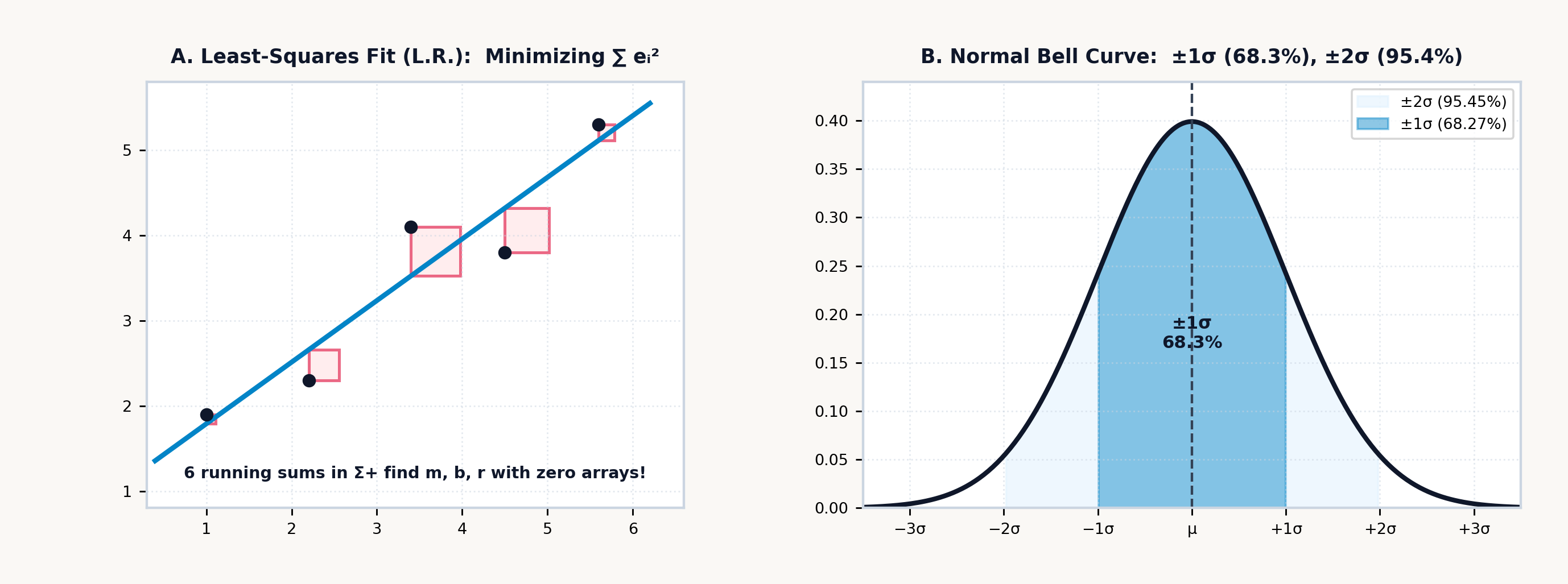
Gauss's least-squares straight line \(\hat{y} = m x + b\) (Figure 9.1) through \(n\) bivariate observations \((x_1, y_1), (x_2, y_2), \dots, (x_n, y_n)\) minimizes the sum of squared vertical residuals \(S(m, b) = \sum_{k=1}^n [y_k - (m x_k + b)]^2\). Setting the partial derivatives \(\frac{\partial S}{\partial b} = -2\sum(y_k - m x_k - b) = 0\) and \(\frac{\partial S}{\partial m} = -2\sum x_k(y_k - m x_k - b) = 0\) expresses the best-fit slope \(m\), vertical intercept \(b\), and Pearson product-moment correlation coefficient \(r \in [-1, +1]\) in terms of the sample standard deviations \(s_x, s_y\) and the sample covariance \(s_{xy} = \frac{1}{n-1}\sum_{k=1}^n (x_k - \bar{x})(y_k - \bar{y})\) (Gauss, 1809):
Both \(m\) and \(r\) are driven by the sample covariance \(s_{xy}\) (\(n\Sigma xy - \Sigma x\,\Sigma y = n(n-1)s_{xy}\)), which turns positive when above-average \(x_k\) pairs with above-average \(y_k\) and negative when one rises as the other falls. Normalizing \(s_{xy}\) by the horizontal variance \(s_x^2\) gives the physical rate of change \(m = s_{xy}/s_x^2\) (in units of \(\Delta y / \Delta x\)), while \(b = \bar{y} - m\bar{x}\) anchors the line through the data centroid \((\bar{x}, \bar{y})\).
Normalizing \(s_{xy}\) instead by the geometric mean of the horizontal and vertical spreads (\(s_x s_y\)) strips away physical units entirely, leaving Pearson's \(r = s_{xy}/(s_x s_y)\) as a dimensionless measure of linear alignment in \([-1, +1]\): \(r = +1\) denotes an exact positive linear law, \(r = -1\) an exact negative linear law, and \(r = 0\) zero linear covariance, while the coefficient of determination \(R^2 = r^2 \in [0, 1]\) measures the exact fraction of total vertical variance \(\sum(y_k - \bar{y})^2\) explained by the linear predictor \(\hat{y} = mx + b\). By the normal equations, a unique non-vertical line exists if and only if at least two entered \((x_k, y_k)\) pairs have distinct horizontal coordinates (\(\sigma_x > 0\)); if all points share the identical \(x\)-coordinate, they stack in a vertical column where \(n\Sigma x^2 - (\Sigma x)^2 = n^2\sigma_x^2\) vanishes.
In streaming least-squares estimation, the individual coordinates \((x_k, y_k)\) never need to be stored in an expanding table: the sample means, Bessel variances, covariance, slope \(m\), intercept \(b\), and correlation \(r\) are determined by six running sufficient statistics: \(\Sigma x, \Sigma y, \Sigma x^2, \Sigma y^2, \Sigma xy,\) and \(n\). Once a transducer is calibrated across reference standards, forward prediction evaluates the expected response \(\hat{y} = mx_0 + b\) at a known stimulus \(x_0\), while inverse prediction inverts the calibration line \(\hat{x} = (y_0 - b)/m\) (whenever \(m \ne 0\)) to recover an unknown physical stimulus from a measured sensor output \(y_0\).
Because a least-squares line is estimated from a finite sample of \(n\) noisy pairs—leaving a vertical residual standard error \(s_e = \sqrt{\frac{1}{n-2}\sum (y_k - \hat{y}_k)^2}\) around the line with \(n - 2\) degrees of freedom and a two-sided Student-\(t\) critical multiplier \(t_{\alpha/2,\,n-2}\)—the fitted line carries sampling uncertainty in both its centroid height \(\bar{y}\) and its tilt \(m\). Combining those independent error sources gives the pointwise confidence half-width \(E_{\text{mean}}(x_0)\) for the mean regression line \(\mathbb{E}[Y \mid x_0]\) and the wider prediction half-width \(E_{\text{pred}}(x_0)\) for a single future measurement \(y_{\text{new}}\) at \(x_0\):
Three independent variance contributions add inside the square root (each scaled by \(s_e^2\)): \(\frac{1}{n}\) captures the vertical uncertainty in the center height \(\bar{y}\) of the data cloud; \(\frac{(x_0 - \bar{x})^2}{(n-1)s_x^2}\) captures the lever-arm tilt uncertainty from the slope \(m\), which vanishes right at the centroid waist \(x_0 = \bar{x}\) and flares outward into a Working–Hotelling hyperbola as \(x_0\) moves toward the horizontal extremes; and the extra \(+1\) in \(E_{\text{pred}}(x_0)\) adds the baseline scatter \(1 \cdot s_e^2\) of a single new observation around the true regression line.
A linear least-squares engine also fits strongly curved physical laws whenever a smooth coordinate change straightens the curve. Across experimental science and engineering, four standard two-parameter regression models (linear, logarithmic, exponential, and power-law)—together with reciprocal and hyperbolic saturation laws—invert via logarithmic or reciprocal mappings: taking the natural logarithm \(\ln(\cdot)\) converts multiplication and exponentiation into addition, and taking the reciprocal \(1/(\cdot)\) turns a saturation ceiling into a linear intercept, transforming the curved trajectory into a line \(Y' = m X' + b\):
| Curve Model Family | Governing Physical Equation | Coordinate Transformation (\(Y', X'\)) | Linearized Equation (\(Y' = m X' + b\)) | Parameter Recovery from Slope \(m\) & Intercept \(b\) |
|---|---|---|---|---|
| 1. Linear | \(y = m x + b\) | \(Y' = y,\quad X' = x\) | \(y = m x + b\) | Slope \(= m\), Intercept \(= b\) |
| 2. Logarithmic | \(y = b + m \ln x\) | \(Y' = y,\quad X' = \ln x\) | \(y = m (\ln x) + b\) | Scale \(= m\), Offset \(= b\) |
| 3. Exponential | \(y = a e^{m x}\) | \(Y' = \ln y,\quad X' = x\) (Semi-Log) | \(\ln y = m x + \ln a\) | Rate \(= m\), Initial \(a = e^b\) |
| 4. Power | \(y = a x^m\) | \(Y' = \ln y,\quad X' = \ln x\) (Log-Log) | \(\ln y = m \ln x + \ln a\) | Exponent \(= m\), Scale \(a = e^b\) |
| 5. Reciprocal | \(\frac{1}{y} = m x + b\) | \(Y' = 1/y,\quad X' = x\) | \(y^{-1} = m x + b\) | Rate \(= m\), Ceiling \(y_0 = 1/b\) |
| 6. Hyperbolic | \(y = \frac{V_{\max} x}{K_m + x}\) | \(Y' = 1/y,\quad X' = 1/x\) (Lineweaver–Burk) | \(\frac{1}{y} = \frac{K_m}{V_{\max}}\frac{1}{x} + \frac{1}{V_{\max}}\) | \(V_{\max} = 1/b\), \(K_m = m \cdot V_{\max}\) |
Across science and engineering, these six coordinate transformations linearize integrated-circuit transistor doubling (Moore, 1965), the barometric altitude formula \(P(h) = P_0 e^{-h/H}\), radioactive decay \(A(t) = A_0 e^{-\lambda t}\), the Arrhenius chemical activation law \(k = A e^{-E_a/(RT)}\) (\(\ln k\) against \(1/T\)), and wind-turbine Betz cubic power scaling \(P = k v^3\) (\(\ln P\) against \(\ln v\)).
9.1.4 Enzyme Saturation Kinetics & Spectrophotometric Calibration
In biochemistry and analytical chemistry, nonlinear saturation curves and exponential optical attenuation reduce to linear calibration models in transformed coordinates.
Under steady-state enzyme kinetics (\(E + S \underset{k_{-1}}{\overset{k_1}{\rightleftharpoons}} ES \overset{k_{\text{cat}}}{\longrightarrow} E + P\)), the initial catalytic reaction velocity \(v_0\) follows a rectangular hyperbola across substrate molarity \([S]\) governed by the Michaelis–Menten equation, which straightens into a line when inverted on both axes:
The saturation ceiling \(V_{\max} = k_{\text{cat}}[E]_{\text{total}}\) represents the maximum turnover velocity when every catalytic site is occupied, while the Michaelis affinity constant \(K_m = (k_{-1} + k_{\text{cat}})/k_1\) marks the exact substrate concentration at which reaction velocity reaches half of that ceiling (\(v_0 = \frac{1}{2}V_{\max}\)). At trace substrate levels (\([S] \ll K_m\)), catalytic sites sit mostly vacant and reaction rate scales linearly with substrate as apparent first-order kinetics \(v_0 \approx (V_{\max}/K_m)[S]\); at high substrate excess (\([S] \gg K_m\)), every active site is occupied and \(v_0\) plateaus asymptotically at the zero-order ceiling \(V_{\max}\). For an assay with \(V_{\max} = 140\text{ }\mu\text{M/min}\) and \(K_m = 5\text{ mM}\) evaluated at \([S] = 15\text{ mM}\) (three times \(K_m\)), dividing \(V_{\max}[S] = 2,100\) by \(K_m + [S] = 20\text{ mM}\) yields an initial velocity of \(v_0 = \mathbf{105\text{ }\mu\text{M/min}}\) (exactly \(\frac{3}{4}V_{\max}\)).
To extract \(V_{\max}\) and \(K_m\) from experimental rate measurements via linear regression, taking the reciprocal of both sides (the Lineweaver–Burk double-reciprocal transformation) inverts the saturation hyperbola into a straight line of \(Y' = 1/v_0\) against \(X' = 1/[S]\), with vertical intercept \(b = 1/V_{\max}\) and slope \(m = K_m / V_{\max}\). When very low substrate readings carry large relative measurement noise—since \(\Delta(1/v_0) \approx -\Delta v_0 / v_0^2\) amplifies small-velocity errors—analysts cross-check using a regression of \(v_0\) against \(v_0/[S]\) or \([S]/v_0 = \frac{1}{V_{\max}}[S] + \frac{K_m}{V_{\max}}\), which weights high-signal measurements more evenly across the concentration range.
Often the substrate or product concentration \([S]\) in such kinetic assays is measured optically via the Beer–Lambert Law. Monochromatic light of incident intensity \(I_0\) passing through an absorbing medium of molar concentration \(c\) and cuvette path length \(b = \ell\) suffers exponential photon attenuation \(I = I_0 10^{-A}\), because each infinitesimal slice \(dx\) absorbs a constant fraction of the photons entering it (\(dI / I = -\ln(10)\varepsilon c\,dx\)), governed by the wavelength-specific molar absorptivity coefficient \(\varepsilon\). Laboratory spectrophotometry linearizes the exponential attenuation law \(I = I_0 10^{-\varepsilon b c}\) into a straight least-squares calibration line by taking the negative base-10 logarithm of optical transmittance \(T = I/I_0\) to define dimensionless decadic absorbance \(A\):
Just as double-reciprocal inversion (\(1/v_0\) vs. \(1/[S]\)) and log-log transformation (\(\ln y\) vs. \(\ln x\)) straighten hyperbolic and power-law kinetics, logging a series of reference concentrations \(c_k\) and measured absorbances \(A_k\) fits the calibration line \(A = (\varepsilon b)c + A_{\text{blank}}\) with slope \(m = \varepsilon b\) and reagent-blank intercept \(b_0 = A_{\text{blank}}\). In an enzymatic \(\text{NADH}\) assay monitored at \(\lambda = 340\text{ nm}\) with molar absorptivity \(\varepsilon = 6,220\text{ L}\cdot\text{mol}^{-1}\cdot\text{cm}^{-1}\) across a standard \(b = \ell = 1\text{ cm}\) quartz cuvette at concentration \(c = 8.5 \times 10^{-5}\text{ mol/L}\), the linear product \(\varepsilon b c\) gives an absorbance of \(A \approx \mathbf{0.529}\) (well within the \(A \in [0.1, 1.5]\) spectrophotometric window where stray light and shot noise are minimized), corresponding to an exponentially attenuated transmittance fraction of \(T = I/I_0 \approx 10^{-0.529} \approx \mathbf{0.296}\) (\(29.6\%\) transmitted light).
9.2 Small-Sample Inference, Rare Events & Diagnostic Uncertainty
Classical Gaussian error theory assumes hundreds or thousands of observations (\(n \to \infty\)), where the Bessel sample standard deviation \(s_x\) has converged so closely to the true population parameter \(\sigma\) that replacing \(\sigma\) with \(s_x\) inside \(z = \frac{\bar{x} - \mu}{\sigma / \sqrt{n}}\) introduces negligible error.
In destructive aerospace metallurgy, semiconductor pilot runs, clinical pharmacology, and industrial quality control, however, testing thousands of specimens is rarely possible; engineers routinely work with small experimental batches of \(n = 4\) to \(10\) samples. When \(n\) is small, the sample standard deviation \(s_x\) fluctuates randomly from batch to batch alongside the sample mean \(\bar{x}\). Whenever a small random sample happens by chance to cluster tightly together, \(s_x\) underestimates \(\sigma\) and inflates the quotient \(t = \frac{\bar{x} - \mu}{s_x / \sqrt{n}}\), causing extreme tail values to occur far more often than Gauss's unit normal distribution predicts.
Published in 1908 by William Sealy Gosset ("Student"), orthogonal spherical geometry in \(n\)-dimensional space accounts for the joint random fluctuation of \(\bar{x}\) and \(s_x\) across \(\nu = n - 1\) degrees of freedom (normalized to unit total probability area by Euler's Gamma function \(\Gamma(x) = \int_0^\infty u^{x-1}e^{-u}\,du\), the continuous extension of the factorial satisfying \(\Gamma(k+1) = k!\)) to yield the small-sample probability density of Student's \(t\)-distribution (Student, 1908):
The leading Gamma-function ratio normalizes the central peak so the integral over \((-\infty, +\infty)\) equals \(1\), while the algebraic factor \(\left(1 + \frac{t^2}{\nu}\right)^{-(\nu+1)/2}\) governs the heavy tails: unlike the Gaussian density \(e^{-z^2/2}\), whose tails decay super-exponentially, Student's \(t\)-density decays as a power law \(|t|^{-(\nu + 1)}\) to protect small-sample inference against lucky tight clusters in \(s_x\) (reducing at \(\nu = 1\) to the Cauchy–Lorentz resonance curve \(\frac{1}{\pi(1+t^2)}\) and converging smoothly back to the Gaussian bell curve \(\frac{1}{\sqrt{2\pi}}e^{-t^2/2}\) as \(\nu \to \infty\) via the compound-interest limit \(\lim_{\nu\to\infty}(1 + t^2/\nu)^{-\nu/2} = e^{-t^2/2}\)).
To test whether the observed sample means \(\bar{x}_1\) and \(\bar{x}_2\) of two small independent experimental groups of sizes \(n_1\) and \(n_2\) and Bessel standard deviations \(s_1\) and \(s_2\) differ significantly (as in ultimate tensile strength coupons of two candidate aerospace titanium alloys), Student's Two-Sample \(t\)-Test first combines the two sample variances into a pooled standard deviation \(s_p\) weighted by their respective degrees of freedom (\(\nu_1 = n_1 - 1\) and \(\nu_2 = n_2 - 1\), yielding \(\nu = n_1 + n_2 - 2\) total degrees of freedom):
Summing the squared deviations \((n_1 - 1)s_1^2 + (n_2 - 1)s_2^2\) from both groups and dividing by the combined degrees of freedom \(n_1 + n_2 - 2\) forms the pooled variance \(s_p^2\). The test statistic \(t\) then acts as a signal-to-noise ratio, comparing the observed separation between the two group averages (\(\bar{x}_1 - \bar{x}_2\)) against the standard error \(s_p\sqrt{1/n_1 + 1/n_2}\) expected from random sampling noise alone. When the two groups have markedly unequal variances (\(s_1^2 \ne s_2^2\)), the Welch–Satterthwaite unpooled statistic \(t = \frac{\bar{x}_1 - \bar{x}_2}{\sqrt{s_1^2/n_1 + s_2^2/n_2}}\) replaces the pooled standard error; for paired before-and-after measurements \((x_{1,k}, x_{2,k})\) on the same \(n\) specimens, accumulating the pairwise differences \(d_k = x_{1,k} - x_{2,k}\) eliminates specimen-to-specimen baseline variance and evaluates the single-sample paired ratio \(t = \frac{\bar{d}}{s_d / \sqrt{n}}\) with \(\nu = n - 1\) degrees of freedom.
9.2.1 Leverage, Error Propagation & the Weibull Bathtub Curve
Three geometric properties of least-squares projection and fatigue survival govern uncertainty analysis and hardware reliability.
First, every least-squares regression line \(\hat{y} = mx + b\) passes through the centroid \((\bar{x}, \bar{y})\) of the data cloud (\(\bar{y} = m\bar{x} + b\)), acting like a rigid mechanical beam balanced on a pin fulcrum at \((\bar{x}, \bar{y})\) and tethered by vertical Hookean springs of stiffness \(k\) to each observation \((x_i, y_i)\). Because torque equals force times lever arm \(|x_i - \bar{x}|\), any datum near the horizontal extremes exerts high statistical leverage \(h_{ii} = \frac{1}{n} + \frac{(x_i - \bar{x})^2}{(n-1)s_x^2}\) on the fitted slope \(m\) (often called the hat-value because it measures how strongly an observation at \(x_i\) pulls the fitted "hat" curve \(\hat{y}\)). In the degenerate two-point case (\(n = 2\)), each endpoint carries maximum leverage \(h_{11} = h_{22} = 1\), forcing the least-squares line to pass exactly through both points (\(r = \pm 1\)) with secant slope \(m = \frac{y_2 - y_1}{x_2 - x_1}\) and turning linear regression into an exact two-point forward and inverse linear interpolator for engineering steam, psychrometric, and standard-atmosphere lookup tables.
Once \(\hat{y} = mx + b\) is fitted across \(n\) pairs, the remaining vertical scatter around the line is measured by the residual standard error \(s_e = \sqrt{\frac{1}{n-2}\sum_{i=1}^n (y_i - \hat{y}_i)^2}\), where \(n - 2\) reflects the two degrees of freedom consumed in estimating both \(m\) and \(b\). By the Pythagorean orthogonality of the least-squares projection, the total sum of squares \((n-1)s_y^2\) decomposes into the explained regression fraction \(r^2\) and the unexplained residual fraction \((1 - r^2)\), allowing \(s_e\) and the standard error of the slope \(\text{SE}(m) = \frac{s_e}{s_x\sqrt{n-1}}\) to be evaluated from the statistical summary quantities without re-scanning the \(n\) points:
Early pocket calculators compressed an entire dataset into six sufficient summary sums (\(\Sigma x, \Sigma y, \Sigma x^2, \Sigma y^2, \Sigma xy, n\)) to compute means, Bessel standard deviations, and linear regression lines in six memory words, but they discarded the individual points \((x_k, y_k)\) the moment they were summed. If an experimenter later needed to plot the scatter cloud on a graphical canvas to check for curvature, or audit which specific measurement caused an unexpected outlier residual, the raw observations were gone. Retaining the individual sample values alongside the six sufficient statistics bridges classical summary accumulation and visual exploratory data analysis, allowing both algebraic moment queries and direct inspection or scatter plotting of the underlying points.
Second, when two noisy measurements \(X \pm \sigma_X\) and \(Y \pm \sigma_Y\) (with linear correlation \(r\)) are combined through a differentiable physical formula \(Z = g(X, Y)\), a small perturbation \(dX\) or \(dY\) shifts the output by Gauss's first-order Taylor differential \(dZ = \frac{\partial g}{\partial X}dX + \frac{\partial g}{\partial Y}dY\). Here the partial derivatives \(\frac{\partial g}{\partial X}\) and \(\frac{\partial g}{\partial Y}\) are the local sensitivity amplification factors—the slopes measuring how strongly the calculated output \(Z\) responds to small wiggles in \(X\) and \(Y\) respectively. Squaring \(dZ\) and averaging across the measurement noise yields the general Law of Error Propagation for the output variance \(\sigma_Z^2\):
Each input variance \(\sigma_X^2\) and \(\sigma_Y^2\) is weighted by the square of its local sensitivity slope, while the cross-term \(2\left(\frac{\partial g}{\partial X}\right)\left(\frac{\partial g}{\partial Y}\right)r\sigma_X\sigma_Y\) adds or subtracts their covariance interaction whenever noise in \(X\) and \(Y\) is correlated (\(r \ne 0\)). For uncorrelated sums and differences \(Z = X \pm Y\) (where \(\frac{\partial g}{\partial X} = 1,\; \frac{\partial g}{\partial Y} = \pm 1,\; r = 0\)), absolute uncertainties add in quadrature (\(\sigma_Z = \sqrt{\sigma_X^2 + \sigma_Y^2}\), matching the Euclidean hypotenuse of a right triangle with legs \(\sigma_X\) and \(\sigma_Y\)); for products and quotients \(Z = X^a Y^b\), relative uncertainties add in quadrature: \(\frac{\sigma_Z}{|Z|} = \sqrt{\left(a\frac{\sigma_X}{X}\right)^2 + \left(b\frac{\sigma_Y}{Y}\right)^2}\). When \(m\) independent sensors of unequal noise variances \(\sigma_1^2, \dots, \sigma_m^2\) measure the same physical quantity \(\mu\), the Gauss–Markov minimum-variance unbiased estimator weights each reading inversely by its error variance (\(w_i = 1/\sigma_i^2\)), yielding the weighted mean \(\bar{x}_w\) with combined fused uncertainty \(\sigma_{\text{fused}} = 1/\sqrt{\sum w_i}\).
Third, while radioactive decay and photon arrivals are memoryless, mechanical ball bearings, aircraft wing spars, and ceramic capacitors accumulate sub-surface cyclic fatigue damage as operating hours \(t\) increase. Derived from weakest-link extreme-value theory, the two-parameter Weibull survival distribution \(R(t)\) (Weibull, 1951) and instantaneous failure hazard rate \(h(t) = -\frac{d}{dt}\ln R(t)\) unify all three stages of the reliability bathtub curve via characteristic scale life \(\eta\) (the age at which \(e^{-1} \approx 36.79\%\) of units survive) and dimensionless shape modulus \(\beta\):
When \(\beta < 1\) (infant mortality / burn-in), latent manufacturing defects fail early and \(h(t)\) decreases with age; when \(\beta = 1\) (random external shocks), \(h(t) = 1/\eta\) is constant and recovers the memoryless exponential law \(R(t) = e^{-t/\eta}\); when \(\beta > 1\) (fatigue wear-out), \(h(t)\) accelerates with age. Inverting \(R(t_{p}) = 1 - p\) gives the \(B_{10}\) bearing rating life \(t_{0.1} = \eta [-\ln(0.9)]^{1/\beta}\) at which \(90\%\) of a fleet survives, while taking the double natural logarithm \(\ln[-\ln R(t)] = \beta \ln t - \beta \ln \eta\) linearizes empirical survival curves into a straight regression line.
9.2.2 Statistical Inference, Rare Events & Experimental Uncertainty
The transition from describing a finite dataset to predicting the behavior of an unseen physical process unites discrete probability, industrial quality control, and Bayesian inverse inference into a single quantitative framework.
When \(n\) independent, identically distributed binary trials each succeed with probability \(p \in [0, 1]\) and fail with probability \(q = 1 - p\), any specific ordered sequence of \(k\) successes and \(n - k\) failures occurs with product probability \(p^k(1 - p)^{n-k}\), and the binomial coefficient \(\binom{n}{k} = \frac{n!}{k!(n-k)!}\) counts how many distinct trajectories share that exact tally, with mean \(\mu = np\) and variance \(\sigma^2 = np(1 - p)\). In semiconductor yield auditing, if a wafer fabrication step carries a per-die defect probability of \(p = 0.25\) across \(n = 10\) test dies, there are \(\binom{10}{3} = 120\) distinct combinations of \(k = 3\) defective dies, and multiplying \(120 \times 0.25^3 \times 0.75^7\) gives a binomial probability of \(P(X = 3) \approx \mathbf{0.25}\) (\(25\%\)).
As the number of opportunities \(n\) in the binomial law grows large while the probability \(p\) of an event in any single micro-interval shrinks toward zero at a constant average arrival rate \(\lambda = np\), the binomial probability \(\binom{n}{k}p^k(1-p)^{n-k}\) converges to the Poisson distribution of rare, memoryless events:
Because a memoryless Poisson process has variance equal to its mean (\(\sigma^2 = \mu = \lambda\)), its root-mean-square fluctuation scales as \(\sqrt{\lambda}\)—the fundamental origin of photon shot noise in optical detectors, radioactive count scatter, cosmic-ray SRAM bit flips, and unscheduled packet arrivals at a network switch. For an avalanche photodiode receiving an average of \(\lambda = 4.2\text{ photons/ms}\), the probability of detecting exactly \(k = 3\) photons in a one-millisecond gate is \(4.2^3 e^{-4.2} / 3! \approx 74.088 \times 0.015 / 6 \approx \mathbf{0.185}\) (\(18.5\%\)).
When a scientist or quality engineer tests whether an empirical histogram of observed counts \(O_1, O_2, \dots, O_k\) across \(k\) categories obeys a hypothesized binomial, Poisson, or Gaussian distribution with expected counts \(E_1, E_2, \dots, E_k\) (and \(p\) distribution parameters such as \(\lambda\), \(\mu\), or \(\sigma\) estimated from the sample itself), the Chi-Square (\(\chi^2\)) Goodness-of-Fit Test sums the squared count discrepancies normalized by each cell's expected variance \(E_i\) across \(\nu = k - 1 - p\) degrees of freedom:
Dividing each squared count discrepancy \((O_i - E_i)^2\) by that cell's expected Poisson variance \(E_i\) places high-count and low-count categories on an equal standardized scale, while the degrees of freedom \(\nu = k - 1 - p\) deduct one constraint for the fixed total sample size \(\sum O_i = \sum E_i = N\) and \(p\) constraints for the fitted parameters.
In industrial manufacturing, statistical process control separates natural, random common-cause noise from actionable assignable-cause mechanical faults. Adjusting a stable lathe after every random common-cause fluctuation (tampering) doubles output variance, while \(\pm 3\sigma_{\bar{x}}\) Shewhart control limits isolate genuine tool wear or fixture slip. To bound the population mean within a confidence margin \(E\) using the two-sided normal critical multiplier \(z_{\alpha/2}\) (\(z_{0.025} \approx 1.96\) for \(95\%\) confidence), and to compare a machine's natural sample spread \(s\) and process center \(\bar{x}\) against engineering blueprint tolerances—the Upper and Lower Specification Limits (\(\text{USL}\) and \(\text{LSL}\))—Six Sigma metrology pairs the potential capability index \(C_p\) with the off-center capability index \(C_{pk}\):
Think of driving a car of width \(6s\) (the \(\pm 3s\) natural spread encompassing \(99.73\%\) of parts) through a garage doorway of total tolerance width \(\text{USL} - \text{LSL}\). The potential capability \(C_p = \frac{\text{USL} - \text{LSL}}{6s}\) compares the doorway width against the \(6s\) car width—telling you whether the car could fit if steered dead center—whereas the actual capability \(C_{pk}\) takes the distance from the off-center process mean \(\bar{x}\) to the nearer doorway wall (\(\text{USL} - \bar{x}\) or \(\bar{x} - \text{LSL}\)) and divides by the \(3s\) half-car width to measure how close the fender is to scraping the nearer wall.
Because the standard error of the mean shrinks as \(s/\sqrt{n}\) in \(E = z_{\alpha/2}\frac{s}{\sqrt{n}}\), quadrupling the sample size \(n\) is required to halve the uncertainty margin \(E\) (for \(n = 49\) alloy tensile specimens with \(s = 8.4\text{ MPa}\) and \(95\%\) normal quantile \(z_{0.025} \approx 1.96\), the standard error is \(8.4 / 7 = 1.2\text{ MPa}\) and the \(95\%\) confidence half-width is \(E \approx \mathbf{2.352\text{ MPa}}\)). In precision grinding where \(\text{USL} = 10.05\text{ mm}\), \(\text{LSL} = 9.95\text{ mm}\), \(\bar{x} = 10.01\text{ mm}\), and \(s = 0.01\text{ mm}\), the distance to the nearer upper boundary is \(\text{USL} - \bar{x} = 0.04\text{ mm}\), yielding \(C_{pk} = 0.04 / (3 \times 0.01) \approx \mathbf{1.333}\), which meets the \(\pm 4\sigma\) (\(63\text{ ppm}\) defect rate) industrial acceptance benchmark.
Finally, when an automated inspection station or clinical assay screens for a true underlying condition \(A\) (such as a sub-surface crack, occurring with prior prevalence \(P(A)\) while defect-free parts \(A'\) make up the complement \(P(A') = 1 - P(A)\)) and flags a part with a positive alarm \(B\), interpreting that alarm requires inverting the detector's true-positive sensitivity \(P(B \mid A)\) and false-positive rate \(P(B \mid A')\) via Bayes's Theorem:
Bayes's fraction divides the true-alarm rate \(P(B \mid A)P(A)\)—the fraction of all parts that are both genuinely defective and trigger an alarm—by the total alarm rate \(P(B \mid A)P(A) + P(B \mid A')P(A')\), which pools true alarms with the false alarms generated by the defect-free majority. This ratio exposes the counterintuitive base-rate fallacy: when ultrasonic non-destructive testing screens turbine blades for a rare sub-surface crack of prior prevalence \(P(A) = 0.01\) (\(P(A') = 0.99\)) using a detector with \(99\%\) true-positive sensitivity (\(P(B \mid A) = 0.99\)) and a \(5\%\) false-positive rate (\(P(B \mid A') = 0.05\)), true-positive alarms occur across \(0.99 \times 1\% = 0.99\%\) of all blades, while false alarms from the vast defect-free population occur across \(0.05 \times 99\% = 4.95\%\) of all blades. Dividing \(0.99\%\) by the total alarm rate \(0.99\% + 4.95\% = 5.94\%\) reveals that a flagged blade has only a \(P(A \mid B) \approx \mathbf{16.7\%}\) posterior probability of carrying an actual crack until confirmed by a secondary orthogonal scan.
9.3 Six Sufficient Statistics: Calibration and Inference on the Stack
An entire dataset of \(n\) paired observations \((x_k, y_k)\) reduces without loss of linear-regression information to six running sums (\(\Sigma x, \Sigma y, \Sigma x^2, \Sigma y^2, \Sigma xy, n\)). Because those six first- and second-order moments form a complete set of sufficient statistics for Gaussian means, Bessel variances, and linear least squares, the SC-32 links the live four-register stack (X, Y, Z, T) to six 64-bit hardware accumulators in indirect memory—sample count \(n\) (R28), linear totals \(\Sigma x\) (R29) and \(\Sigma y\) (R30), sums of squares \(\Sigma x^2\) (R31) and \(\Sigma y^2\) (R32), and cross-product \(\Sigma xy\) (R33)—so means, standard deviations, and inverse calibration estimates can be queried without re-entering data arrays:
- Resetting, Logging, & Inspecting Observations (
[↰] [CLEAR],[Σ+],[↰] [Σ-],[↰] [REGS]): Pressing[↰] [CLEAR]offers[CLSTAT]([CLΣ]) to zero all six statistical registers (R28–R33) and clear the raw data log. When logging a bivariate observation \((x_k, y_k)\), placing the vertical response \(y_k\) into Register \(Y\) and the horizontal predictor \(x_k\) into Register \(X\) before pressing[Σ+]aligns the display registers \((Y, X)\) with the \((y, x)\) axes of the coordinate plane, displays the updated sample count \(n\) in Register \(X\) with stack lift disabled (leaving the priorLASTXregister undisturbed), and records up to 50 individual sample values inDATA0–DATA49(indirect slotsR40–R89, inspectable read-only via[↰] [REGS]\(\to\)DATA, and plotted in the companion app via[↱] [PLOT]whenΣ+data is present with no stored equations;PLOTis excluded from physical hardware firmware by design for examination compliance). - Statistical Softkey Menus (
[↱] [SUMS],[↱] [x̄,ȳ],[↱] [s,σ],[↱] [L.R.]): Accessed via Right Shift[↱]across the top scientific row—[↱] [SUMS]on[Σ+],[↱] [x̄,ȳ]on[yˣ],[↱] [s,σ]on[1/x], and[↱] [L.R.]on[LN]—the four statistical menus remap the six top-row softkey slots (Slot 1throughSlot 6):
| Sub-Menu | Physical Key | Slot 1 |
Slot 2 |
Slot 3 |
Slot 4 |
Slot 5 |
Slot 6 |
|---|---|---|---|---|---|---|---|
1. Sums ([↱] [SUMS]) |
[Σ+] |
\(\Sigma x\) | \(\Sigma y\) | \(\Sigma x^2\) | \(\Sigma y^2\) | \(\Sigma xy\) | \(n\) |
2. Means ([↱] [x̄,ȳ]) |
[yˣ] |
\(\bar{x}\) | \(\bar{y}\) | \(\bar{x}_w\) | — | — | — |
3. Std Dev ([↱] [s,σ]) |
[1/x] |
\(s_x\) | \(s_y\) | \(\sigma_x\) | \(\sigma_y\) | — | — |
4. Regression ([↱] [L.R.]) |
[LN] |
\(\hat{y}\) | \(\hat{x}\) | \(r\) | \(m\) | \(b\) | — |
If a keystroke slip on the sixth data pair \((x = 15, y = 3.5)\) transposes \(y\) into \((x = 15, y = 5.3)\) when the sample count is \(n = 6\), staging \((Y = 5.3, X = 15)\) and pressing Σ- (left-shifted on Σ+) removes the erroneous point from all six accumulators (decrementing \(n\) to \(5\)) so the corrected pair \((Y = 3.5, X = 15)\) can be spliced in with Σ+ without disturbing the first five observations. Following HP-32SII statistical stack-lift semantics (HP, 1991), [Σ+] and [↰] [Σ-] leave stack lift disabled when writing the sample count \(n\) into Register \(X\). Consequently, the first statistical softkey tapped immediately after [Σ+]—whether x̄, ȳ, or x̄w in x̄,ȳ, sx, sy, σx, or σy in s,σ, r, m, or b in L.R., or any accumulator in SUMS—overwrites the sample count \(n\) in Register \(X\) and enables stack lift. Tapping a second statistical softkey (such as ȳ right after x̄, or sy right after sx) then lifts the first statistic into Register \(Y\) and places the second statistic in Register \(X\), while [ŷ] and [x̂] consume the stimulus \(x_0\) or response \(y_0\) in Register \(X\) to return the linear prediction \(\hat{y}(x_0)\) or \(\hat{x}(y_0)\) in Register \(X\).
9.3.1 Univariate & Weighted Accumulation: Sensor Fusion and Six Sigma Control
In observatory astrometry and shop-floor metrology, these weighted-mean and process-capability estimators feed into subsequent stack arithmetic.
For inverse-variance weighted sensor fusion (\(\bar{x}_w = \Sigma xy / \Sigma y\)), three observatory instruments measure an astrometric parallax angle—\(x_1 = 10\text{ mas}\), \(x_2 = 25\text{ mas}\), and \(x_3 = 45\text{ mas}\)—with inverse-variance precision weights \(w_i = 1/\sigma_i^2\) equal to \(w_1 = 40\), \(w_2 = 60\), and \(w_3 = 20\text{ mas}^{-2}\). Clearing the accumulators and loading each weight \(w_i\) into Register \(Y\) and measurement \(x_i\) into Register \(X\) before accumulating stores \(\Sigma(w_i x_i) = 2,800\) inside R33 (\(\Sigma xy\)) and \(\Sigma w_i = 120\) inside R30 (\(\Sigma y\)). Querying \(\bar{x}_w\) from the means menu returns the minimum-variance fused estimate \(\bar{x}_w = \frac{\Sigma xy}{\Sigma y} = \frac{2800}{120} \approx \mathbf{23.333\text{ mas}}\), while querying \(\Sigma y\) from the sums menu recalls the combined precision weight \(\mathbf{120\text{ mas}^{-2}}\), whose reciprocal square root gives the fused standard error \(\sigma_{\text{fused}} = 1/\sqrt{120} \approx \mathbf{0.091\text{ mas}}\).
In a CNC grinding cell producing bearing shafts specified at \(25 \pm 0.1\text{ mm}\) (\(\text{LSL} = 24.9\text{ mm}\), \(\text{USL} = 25.1\text{ mm}\)), accumulating ten measured shaft diameters (\(25.02, 25.04, 25.01, 25.03, 25.05, 25.02, 25, 25.04, 25.03,\) and \(25.06\text{ mm}\)) yields a sample mean of \(\bar{x} = \mathbf{25.03\text{ mm}}\) and a Bessel sample standard deviation of \(s_x \approx \mathbf{0.018\text{ mm}}\) (or, by shift-invariance \(s_{x-c} = s_x\), accumulating only the hundredths of a millimeter \(2, 4, 1, 3, 5, 2, 0, 4, 3, 6\) yields \(\bar{d} = 3\) and \(s_d \approx 1.826\), corresponding to the unrounded \(s_x = s_d / 100 \approx 1.826 \times 10^{-2}\text{ mm}\) in Register \(X\), in half the keystrokes while avoiding floating-point cancellation). Dividing the \(0.2\text{ mm}\) tolerance width by \(6s_x\) (using the unrounded \(s_x\) in Register \(X\)) gives a potential capability of \(C_p \approx \mathbf{1.826}\), while comparing \(\bar{x} = 25.03\text{ mm}\) against the closer upper limit \(\text{USL} = 25.1\text{ mm}\) via \((\text{USL} - \bar{x})/(3s_x)\) gives \(C_{pk} \approx \mathbf{1.278}\).
That divergence between \(C_p \approx 1.826\) and \(C_{pk} \approx 1.278\) provides an immediate shop-floor diagnosis: the lathe spindle is mechanically tight enough for Six Sigma production (\(C_p > 1.33\)), but thermal tool growth has shifted the process center \(+0.03\text{ mm}\) toward the upper limit, which calls for a \(-0.03\text{ mm}\) tool-offset compensation rather than a spindle rebuild. For a Shewhart \(\bar{X}\)-chart centered at \(\bar{\bar{X}} = 50\text{ mm}\) with subgroup range \(\bar{R} = 0.4\text{ mm}\) and \(n = 5\) subgroup factor \(A_2 \approx 0.577\), the control half-width is \(A_2\bar{R} \approx 0.231\text{ mm}\), placing the Lower and Upper Control Limits at \(\text{LCL} \approx \mathbf{49.769\text{ mm}}\) and \(\text{UCL} \approx \mathbf{50.231\text{ mm}}\) (where recalling the preserved last operand recovers the half-width \(0.231\) after subtracting from \(50\) so doubling and adding steps straight from \(\text{LCL}\) to \(\text{UCL}\)).
9.3.2 Bivariate Linear Calibration: Pressure Transducers and Working–Hotelling Bands
The four dead-weight calibration points of a piezoresistive pressure sensor—\(10\text{ kPa}\) at \(1.25\text{ V}\), \(20\text{ kPa}\) at \(2.45\text{ V}\), \(30\text{ kPa}\) at \(3.8\text{ V}\), and \(40\text{ kPa}\) at \(4.95\text{ V}\)—establish the standard bivariate \((Y = y_k,\; X = x_k)\) entry and linear regression workflow on the stack:
| Keystroke | Register T | Register Z | Register Y | Register X | What Happens on the Stack |
|---|---|---|---|---|---|
[CLΣ] 1.25 [ENTER] 10 [Σ+] |
\(0\) | \(0\) | \(1.25\) | \(1\) | Clear accumulators; log Point 1 (\(10\text{ kPa}, 1.25\text{ V};\; n = 1\)) |
2.45 [ENTER] 20 [Σ+] |
\(0\) | \(1.25\) | \(2.45\) | \(2\) | Log Point 2 (\(20\text{ kPa}, 2.45\text{ V};\; n = 2\)) |
3.8 [ENTER] 30 [Σ+] |
\(1.25\) | \(2.45\) | \(3.8\) | \(3\) | Log Point 3 (\(30\text{ kPa}, 3.8\text{ V};\; n = 3\)) |
4.95 [ENTER] 40 [Σ+] |
\(2.45\) | \(3.8\) | \(4.95\) | \(4\) | Log Point 4 (\(40\text{ kPa}, 4.95\text{ V};\; n = 4\)) |
[↱] [L.R.] [m] |
\(2.45\) | \(3.8\) | \(4.95\) | \(0.125\) | Slope \(m \approx 0.125\text{ V/kPa}\) overwrites \(n = 4\) in \(X\) (lift neutral after Σ+) |
25 [↱] [L.R.] [ŷ] 4 [↱] [L.R.] [x̂] |
\(4.95\) | \(0.125\) | \(3.113\) | \(32.129\) | Forward \(\hat{y}(25) \approx 3.113\text{ V}\) in \(Y\); inverse \(\hat{x}(4) \approx 32.129\text{ kPa}\) in \(X\) |
Once those four pairs are committed, the six accumulators hold \(\Sigma x = 100\), \(\Sigma y = 12.45\), \(\Sigma x^2 = 3,000\), \(\Sigma y^2 \approx 46.508\), \(\Sigma xy = 373.5\), and \(n = 4\). Querying the linear regression menu yields a transducer sensitivity slope of \(m \approx \mathbf{0.125\text{ V/kPa}}\), a zero-pressure intercept of \(b = \mathbf{0\text{ V}}\), and a Pearson correlation of \(r \approx \mathbf{1}\) (\(R^2 \approx 0.999\), explaining \(99.9\%\) of variance). Evaluating forward prediction \(\hat{y}\) at \(x_0 = 25\text{ kPa}\) forecasts a sensor output of \(\approx \mathbf{3.113\text{ V}}\), and evaluating inverse prediction \(\hat{x}\) at a measured output of \(y_0 = 4\text{ V}\) lifts \(3.113\text{ V}\) into Register \(Y\) while recovering the unknown line pressure \(\approx \mathbf{32.129\text{ kPa}}\) in Register \(X\).
At the four-point transducer centroid waist \(x_0 = \bar{x} = 25\text{ kPa}\), where the \((x_0 - \bar{x})^2\) tilt term of the Working–Hotelling hyperbolic envelope vanishes, the residual standard error \(s_e \approx 0.058\text{ V}\) and two-sided Student-\(t\) critical quantile \(t_{0.025, 2} \approx 4.303\) give a mean-line confidence margin of \(E_{\text{mean}} = t_{0.025,2} \cdot s_e / \sqrt{4} \approx \mathbf{0.125\text{ V}}\) (\(3.113 \pm 0.125\text{ V}\)), while \(E_{\text{pred}} = t_{0.025,2} \cdot s_e \sqrt{1 + 1/4} = \sqrt{5}\,E_{\text{mean}}\) gives the single-observation prediction margin \(E_{\text{pred}} \approx \mathbf{0.28\text{ V}}\) (\(3.113 \pm 0.28\text{ V}\)).
Because any two points determine an exact secant line with \(r = \pm 1\), logging two adjacent saturated-steam table rows (\(T_1 = 110^\circ\text{C}\) at \(P_1 = 143.27\text{ kPa}\) and \(T_2 = 120^\circ\text{C}\) at \(P_2 = 198.53\text{ kPa}\)) with \((Y = P,\; X = T)\) turns \(\hat{y}\) and \(\hat{x}\) into a reusable two-point table interpolator: querying \(\hat{y}\) at \(T = 114^\circ\text{C}\) interpolates \(P = \mathbf{165.374\text{ kPa}}\), while querying \(\hat{x}\) at \(P = 180\text{ kPa}\) inverts the table to \(T \approx \mathbf{116.647^\circ\text{C}}\) without re-entering the table bounds.
9.3.3 Spectrophotometric Inverse Prediction & Nonparametric Rank Correlation
In analytical and environmental chemistry, inverse regression (\(\hat{x}\)) applies to Beer–Lambert UV-Vis spectrophotometry (\(A = \varepsilon b C + A_{\text{blank}}\)). When a water-quality chemist calibrates a \(b = 1\text{ cm}\) cuvette at \(\lambda = 510\text{ nm}\) across four iron(II)–phenanthroline standards—\(C_1 = 1\text{ mg/L}\) (\(A_1 = 0.198\)), \(C_2 = 2\text{ mg/L}\) (\(A_2 = 0.395\)), \(C_3 = 3\text{ mg/L}\) (\(A_3 = 0.594\)), and \(C_4 = 4\text{ mg/L}\) (\(A_4 = 0.791\))—accumulation of each \((A_i, C_i)\) pair confirms Beer's law linearity (\(r \approx \mathbf{1}\), absorptivity slope \(m \approx \mathbf{0.198\text{ L/mg}}\), blank offset \(b_0 \approx \mathbf{0}\)) and inverts an unknown groundwater sample's absorbance \(A_{\text{unk}} = 0.465\) to \(\hat{C} \approx \mathbf{2.351\text{ mg/L}}\).
When variables are ordinal rankings or follow a monotonic nonlinear relationship, Spearman's rank correlation coefficient \(r_s = 1 - \frac{6\sum d_i^2}{n(n^2 - 1)}\) evaluates Pearson's correlation across the integer ranks \((R_{x,i}, R_{y,i})\) with rank discrepancies \(d_i = R_{x,i} - R_{y,i}\). Across \(n = 5\) ceramic coatings ranked on Mohs scratch hardness versus wear lifetime with rank differences \(d = (1, -1, 2, -1, -1)\), the squared discrepancies sum to \(\sum d_i^2 = 1 + 1 + 4 + 1 + 1 = 8\)—well below the uncorrelated expectation \(n(n^2 - 1)/6 = 20\) (\(r_s = 0\)) and the antipodal reversal sum \(n(n^2 - 1)/3 = 40\) (\(r_s = -1\)). Dividing the numerator \(6\sum d_i^2 = 48\) by \(n(n^2 - 1) = 5(24) = 120\) isolates the discordance penalty \(0.4\), and subtracting from unity yields Spearman's rank correlation \(r_s = \mathbf{+0.6}\).
9.3.4 Bell Curves, Small-Sample \(t\)-Tests & Survival Odds
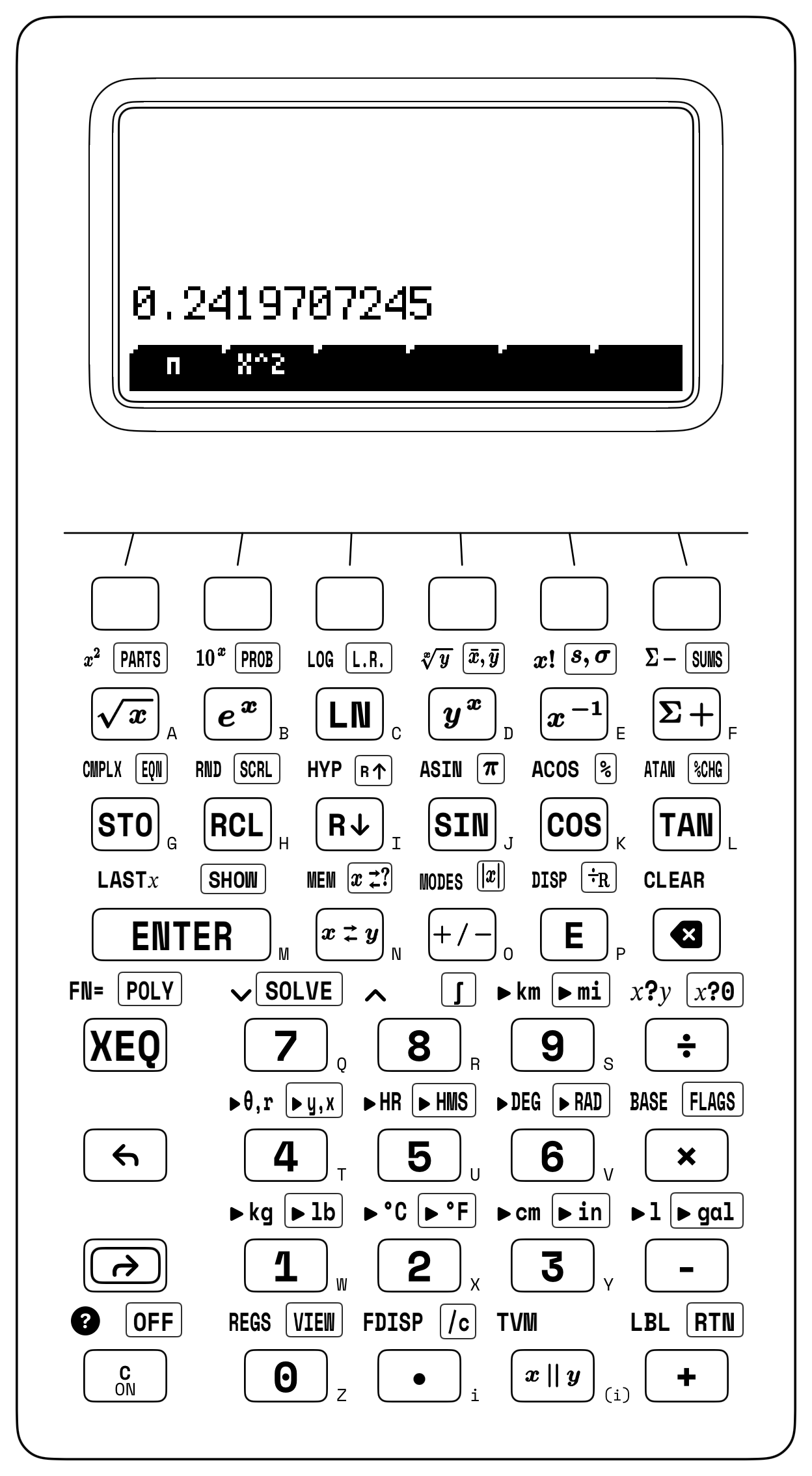
For the Gaussian Normal PDF \(f(x; \mu, \sigma) = \frac{1}{\sigma\sqrt{2\pi}}\exp\!\left(-\frac{(x-\mu)^2}{2\sigma^2}\right)\) at \(x = 115\) with \(\mu = 100\) and \(\sigma = 15\) (\(z = +1\), one standard deviation above the mean), postfix evaluation parks the intermediate exponential factor in the upper registers \(Z\) and \(T\) while the lower registers build the normalization denominator. First, squaring the deviation \((115 - 100)^2 = 225\), dividing by \(2\sigma^2 = 450\), and exponentiating \(-0.5\) leaves the unnormalized bell height \(e^{-0.5} \approx 0.607\) in Register \(X\). Staging \(\sigma = 15\), \(2\), and \(\pi\) then lifts \(e^{-0.5}\) into Registers \(Z\) and \(T\) while \(\sigma\sqrt{2\pi} \approx 37.599\) forms in Register \(X\), so a single division delivers \(f(115; 100, 15) \approx \mathbf{0.016}\) (and multiplying by \(\sigma = 15\) recovers the unit normal height \(\phi(1) \approx \mathbf{0.242}\), Figure 9.2).
To evaluate the cumulative normal integral \(\Phi(1) = 0.5 + \frac{1}{\sqrt{2\pi}}\int_0^{1} e^{-t^2/2}\,dt\) via numerical quadrature, recall that the left half of the symmetric bell curve from \(-\infty\) to \(0\) encloses an exact area of \(0.5\). Integrating the unnormalized kernel \(e^{-x^2/2}\) from \(a = 0\) to \(b = 1\) yields \(\approx 0.856\); dividing by \(\sqrt{2\pi} \approx 2.507\) isolates the half-bell area \(\approx 0.341\) from the mean to \(+1\sigma\), and adding \(0.5\) gives \(\Phi(1) \approx \mathbf{0.841}\) (\(84.1\%\), while doubling the central slice \(2 \times 0.341 \approx \mathbf{0.683}\) confirms the \(\pm 1\sigma\) Empirical Rule of \(68.27\%\)).
In Student's Two-Sample \(t\)-Test (\(\nu = n_1 + n_2 - 2 = 16\)) comparing Titanium Alloy A (\(n_1 = 8\) coupons, \(\bar{x}_1 = 450\text{ MPa}\), \(s_1 = 12.5\text{ MPa}\)) against Alloy B (\(n_2 = 10\) coupons, \(\bar{x}_2 = 468\text{ MPa}\), \(s_2 = 14\text{ MPa}\)), Alloy A's sum of squared deviations \((n_1 - 1)s_1^2 = 7(12.5^2) = 1,093.75\text{ MPa}^2\) combines with Alloy B's \((n_2 - 1)s_2^2 = 9(14^2) = 1,764\text{ MPa}^2\) to form \(2,857.75\text{ MPa}^2\). Dividing by \(\nu = 16\) and taking the square root yields the pooled standard deviation \(s_p \approx \mathbf{13.365\text{ MPa}}\) (weighted \(9:7\) toward the larger 10-coupon batch). Multiplying \(s_p\) by \(\sqrt{1/8 + 1/10} \approx 0.474\) gives the two-sample standard error \(\text{SE} \approx \mathbf{6.339\text{ MPa}}\), and dividing the mean difference \(\bar{x}_1 - \bar{x}_2 = -18\text{ MPa}\) by \(\text{SE}\) yields \(t \approx \mathbf{-2.839}\), which exceeds the two-sided \(95\%\) critical threshold \(t_{0.025, 16} \approx 2.12\) in magnitude and confirms that Alloy B's higher tensile strength is statistically significant.
For a high-speed spindle bearing operating at \(t = 3,000\text{ hr}\) with Weibull characteristic life \(\eta = 5,000\text{ hr}\) and wear-out shape modulus \(\beta = 1.8 > 1\), the normalized age is \(t/\eta = 0.6\), its Weibull hazard power is \((0.6)^{1.8} \approx 0.399\), and the survival probability is \(R(3,000) \approx \exp(-0.399) \approx \mathbf{0.671}\) (\(67.1\%\) survival, or \(32.9\%\) cumulative failure risk).
9.3.5 Coordinate-Transformed Curve Fitting: Power Laws, Kinetics & Activation Energy
Under the log-log transformation (\(\ln P = m\ln v + \ln k\)) for the wind-turbine power law \(P = kv^m\) across four wind-tunnel test points—\((v_1 = 4\text{ m/s}, P_1 = 16\text{ kW})\), \((6, 54)\), \((8, 128)\), and \((10, 250)\)—both output power \(P\) and wind speed \(v\) transform via the natural logarithm on the stack before accumulating each pair. Because executing a unary operator like the natural logarithm or reciprocal terminates digit entry and arms automatic stack lift, typing the horizontal coordinate \(v_i\) after taking \(\ln P_i\) lifts \(\ln P_i\) into Register \(Y\), so taking \(\ln v_i\) and accumulating logs the transformed pair \((\ln v_i, \ln P_i)\) with no intervening ENTER keystroke. Across those four wind-tunnel points, querying the regression slope recovers the exact Betz cubic exponent \(m = \mathbf{3}\), while exponentiating the intercept \(b \approx -1.386\) recovers the aerodynamic scale constant \(k = e^b = \mathbf{0.25\text{ kW/(m/s)}^3}\), forecasting \(P(12) = 0.25 \times 12^3 = \mathbf{432\text{ kW}}\) at \(v = 12\text{ m/s}\).
In a double-reciprocal Lineweaver–Burk enzyme assay (\(1/v_0\) vs. \(1/[S]\)) across four substrate-velocity pairs \(([S]_k, v_k)\) of \((2\text{ mM}, 0.182\text{ }\mu\text{M/min})\), \((4, 0.286)\), \((8, 0.4)\), and \((16, 0.471)\), inverting each reaction velocity \(v_k\) and substrate molarity \([S]_k\) into its reciprocal prior to accumulation yields a reciprocal intercept of \(b = 1/V_{\max} \approx 1.576\) (\(V_{\max} = 1/b \approx \mathbf{0.635\text{ }\mu\text{M/min}}\)) and a slope of \(m = K_m/V_{\max} \approx 7.798\), recovering the half-saturation Michaelis constant \(K_m = m \cdot V_{\max} \approx \mathbf{4.948\text{ mM}}\).
Semi-log radioactive decay fits (\(\ln A(t)\) against untransformed time \(t\)) extract the decay constant \(\lambda = -m\) (\(\lambda \approx \mathbf{0.116\text{ hr}^{-1}}\) and clinical half-life \(t_{1/2} = \ln 2 / \lambda \approx \mathbf{6\text{ hr}}\) for technetium-99m) and initial activity \(A_0 = e^b\), while pairing \(\ln k\) with reciprocal absolute temperature \(1/T\) linearizes the Arrhenius chemical rate law \(k = A\exp(-E_a / RT)\) so that multiplying the negated slope \(-m = E_a / R\) by the universal gas constant \(R \approx 8.314\text{ J/(mol}\cdot\text{K)}\) recovers the molar activation energy barrier \(E_a\).
9.3.6 Try It on the Stack
- Michaelis–Menten Enzyme Velocity via Last-Argument Reuse: For an enzyme assay with \(V_{\max} = 120\,\mu\text{M/min}\) and \(K_m = 4.2\text{ mM}\) at substrate concentration \(c = 8.5\text{ mM}\), evaluate \(v_0 = \frac{V_{\max}c}{K_m + c}\) by forming \(120 \times 8.5 = 1,020\), recalling \(c = 8.5\) via
LASTXto add \(K_m = 4.2\), and dividing. (Verified Register \(X\) result: \(v_0 \approx \mathbf{80.315\,\mu\text{M/min}}\).) - Poisson Rare-Event Arrival Probability: Evaluate the Poisson probability \(P(X = 6) = \frac{\lambda^6 e^{-\lambda}}{6!}\) for an optical receiver averaging \(\lambda = 4.5\text{ photons/gate}\) by raising \(\lambda = 4.5\) to the \(6\text{th}\) power, recalling \(6\) from
LASTXto take its factorial \(6! = 720\) and divide, and multiplying by \(e^{-4.5}\). (Verified Register \(X\) result: \(P(X = 6) \approx \mathbf{0.128}\), or \(12.812\%\).) - Symmetric \(95\%\) Confidence Interval Bounds: For a sample mean \(\bar{x} = 84.625\text{ MPa}\) with standard error \(s_{\bar{x}} = 1.35\text{ MPa}\) and normal quantile \(z = 1.96\), subtract the margin \(E = 1.96 \times 1.35 = 2.646\text{ MPa}\) from \(\bar{x}\) to obtain the lower confidence bound, then restore \(E\) via
LASTX, double it, and add to step to the upper bound. (Verified Register \(X\) results: lower bound \(\mathbf{81.979\text{ MPa}}\) and upper bound \(\mathbf{87.271\text{ MPa}}\).)