Chapter 8: Central Differences, Richardson Extrapolation & Romberg Quadrature
In 1910, while analyzing finite-difference stresses in masonry dams and formulating numerical weather prediction, the English physicist Lewis Fry Richardson identified an algebraic cancellation principle that reshaped numerical calculus (Richardson, 1911): whenever a finite-step approximation to a derivative or an integral carries a truncation error that scales with a known power of the step size \(h\), evaluating the approximation at two step sizes (\(h\) and \(h/2\)) allows the leading error term to be canceled. Generalized into a recursive triangular tableau by Werner Romberg in 1955 (Romberg, 1955), Richardson's extrapolation principle turns simple symmetric secants and flat-topped trapezoids into high-order numerical engines.
Root-finding locates the isolated point where a static function crosses zero; in a moving physical system, forces and rates of change vary continuously from instant to instant. At Launch Complex 39A at Cape Canaveral, when the five Rocketdyne F-1 engines ignite beneath the Apollo Saturn V moon rocket, the first-stage turbopumps deliver fifteen metric tons of kerosene and liquid oxygen per second into the combustion chambers. As hundreds of tons of propellant are expelled through the nozzles, the vehicle mass decreases while engine thrust increases in the thinning upper atmosphere, so acceleration climbs from \(1.25\,g\) at liftoff to \(4.5\,g\) just before staging.
Continuous motion is governed by two complementary operations—the derivative and the definite integral—linked as inverses by the Fundamental Theorem of Calculus. The derivative \(\frac{df}{dt}\) measures the instantaneous rate of change: if \(x(t)\) is the altitude of the Saturn V at time \(t\), its derivative \(v(t) = \frac{dx}{dt}\) is the instantaneous vertical velocity, and the derivative of velocity \(a(t) = \frac{dv}{dt}\) is the instantaneous acceleration. In the reverse direction, the definite integral \(\int_a^b f(t)\,dt\) measures cumulative change across an interval: integrating the area beneath the acceleration curve from ignition (\(t = 0\)) to first-stage burnout (\(t = T\)) recovers the total velocity gained by the spacecraft:
8.1 Symmetric Central Differences & Richardson Extrapolation
A digital instrument evaluates the instantaneous slope (derivative) \(f'(x)\) of a function at a point \(x\) from finite differences without symbolic algebra.
In an introductory calculus course, the derivative is defined by stepping a small distance \(h\) forward to \(x + h\) and computing the difference quotient of the one-sided forward difference:
A one-sided forward difference introduces systematic first-order bias on curved functions. On a curve that bends upward like a parabola (\(f''(x) > 0\)), the secant chord from \(x\) to \(x + h\) is steeper than the true tangent line at \(x\) because the curve rises more rapidly to the right of \(x\). By the Taylor series expansion:
Subtracting \(f(x)\) and dividing by \(h\) leaves a one-sided curvature error of \(+\frac{1}{2}f''(x)h\) that diminishes only linearly with step size—written in Landau big-O notation as \(\mathcal{O}(h)\), where \(\mathcal{O}(h^k)\) denotes a truncation error that shrinks in proportion to \(h^k\) as \(h \to 0\). If one attempts to reduce that \(\mathcal{O}(h)\) truncation error by choosing a tiny step size like \(h = 10^{-11}\), then \(f(x + h)\) and \(f(x)\) agree to their first eleven digits, and subtracting them destroys most of the floating-point precision through catastrophic cancellation.
Geometric symmetry around the point \(x\) eliminates that first-order bias. A symmetric stencil straddles the point \(x\) by stepping backward to \(x - h\) and forward to \(x + h\):
Subtracting the second expansion from the first and dividing by the total span \(2h\) yields the Central Difference Formula:
Stepping equally to the right and left of \(x\) over the span \(2h\) causes the even \(+\frac{1}{2}f''(x)h^2\) curvature terms on the two sides to share the same sign and cancel to zero upon subtraction. Geometrically, the chord joining \((x - h, f(x - h))\) and \((x + h, f(x + h))\) runs nearly parallel to the true tangent line at \(x\), and for any parabola \(f(x) = ax^2 + bx + c\), where the third derivative \(f'''(x) = 0\), the central difference is exact for any step size \(h\).
Choosing the step size \(h\) on a digital processor requires balancing two opposing error sources governed by machine epsilon \(\varepsilon_{\text{mach}} \approx 2.22 \times 10^{-16}\) (the smallest relative spacing between adjacent 64-bit floating-point numbers). If \(h\) is too wide, the secant chord misses the third-order S-bend of the curve, incurring a truncation error \(E_{\text{trunc}} \approx \frac{1}{6}|f'''(x)|h^2\) that grows with \(h^2\). If \(h\) is too narrow, \(f(x + h)\) and \(f(x - h)\) become nearly identical and their subtraction loses guard digits, incurring a roundoff cancellation error \(E_{\text{round}} \approx \frac{\varepsilon_{\text{mach}}|f(x)|}{h}\) that grows with \(1/h\). Differentiating the combined error \(E(h) = \frac{1}{6}|f'''(x)|h^2 + \frac{\varepsilon_{\text{mach}}|f(x)|}{h}\) with respect to \(h\) and setting the derivative to zero locates the sweet-spot step size \(h_{\text{opt}}\) where quadratic truncation error and inverse-step roundoff error meet:
Because \(h^2\) truncation and \(\varepsilon_{\text{mach}}/h\) roundoff differ by three powers of \(h\), their crossover scales as the cube root of machine epsilon (\(\varepsilon_{\text{mach}}^{1/3} \approx 10^{-5}\)), delivering ten to eleven significant digits of derivative accuracy in just two function evaluations: the forward point \(f(x + h)\) and the backward point \(f(x - h)\), whose difference divided by \(2h\) gives the tangent slope.
Whereas subtracting \(f(x+h)\) and \(f(x-h)\) isolates the first derivative, adding them and subtracting \(2f(x)\) cancels the odd terms \(\pm f'(x)h\) and \(\pm\frac{1}{6}f'''(x)h^3\) in Taylor's expansion—leaving the fourth derivative \(f^{(4)}(x)\) as the leading error—and isolates the second derivative \(f''(x)\) (concavity / flexural curvature):
Regrouping the second difference as \([f(x + h) - f(x)] - [f(x) - f(x - h)]\) measures the change in step-change—the forward vertical rise from \(x\) to \(x + h\) minus the backward vertical rise from \(x - h\) to \(x\) (or twice the amount by which the midpoint average \(\frac{1}{2}[f(x+h) + f(x-h)]\) sits above the center value \(f(x)\))—and dividing by \(h^2\) yields the local curvature \(f''(x)\). Because dividing by \(h^2\) amplifies floating-point rounding error as \(\varepsilon_{\text{mach}}/h^2\), balancing it against the \(\frac{1}{12}f^{(4)}(x)h^2\) truncation term shifts the optimal step size for second derivatives to the fourth root of machine epsilon, \(h_{\text{opt}} \approx \varepsilon_{\text{mach}}^{1/4} \approx 10^{-4}\).
In mechanical engineering, derivatives in polar coordinates govern a centrifugal flyball governor regulating rotational speed via negative feedback. When a flyweight of mass \(m\) rotates at angular speed \(\omega\) along a curved cam slot \(r(\theta)\), the flyweight moves tangentially at speed \(v_\theta = r\omega\) while sliding radially outward at speed \(\dot{r} = \omega\frac{dr}{d\theta}\). Combining those two perpendicular velocity components via the Pythagorean theorem (\(v^2 = \dot{r}^2 + (r\omega)^2\)) yields its kinetic energy \(E_k = \frac{1}{2}m\omega^2\left[\left(\frac{dr}{d\theta}\right)^2 + r(\theta)^2\right]\) at any cam angle \(\theta\).
8.1.1 Five-Point Stencil Acceleration via Richardson Extrapolation
Richardson's extrapolation principle (Richardson, 1911) applies directly to the even-power Taylor error series of the central-difference derivative \(D(h)\) (with error coefficients \(c_1 = \frac{1}{6}f'''(x)\) and \(c_2 = \frac{1}{120}f^{(5)}(x)\)):
Because the leading error \(c_1 h^2\) scales with the square of the step size \(h\), evaluating the central difference at step \(h\) (\(D(h)\)) and at twice the step \(2h\) (\(D(2h)\), whose \(h^2\) error is \(4\times\) larger) cancels the \(h^2\) error via \(\frac{4 D(h) - D(2h)}{3}\):
This five-point stencil (\(-1,\; +8,\; 0,\; -8,\; +1\) divided by \(12h\)) combines two central differences at \(h\) and \(2h\) in the ratio \(\frac{4}{3}\) and \(-\frac{1}{3}\), which eliminates the third-derivative error \(\frac{1}{6}f'''(x)h^2\) and achieves fourth-order accuracy \(\mathcal{O}(h^4)\). Evaluating \(f(x) = \sin x\) at \(x_0 = 1\text{ rad}\) (where the exact derivative is \(\cos(1) \approx \mathbf{0.54}\)) using even a deliberately coarse step \(h = 0.1\text{ rad}\) (\(2h = 0.2\text{ rad}\)) yields \(D(0.1) \approx 0.539\) and \(D(0.2) \approx 0.537\), whose Richardson combination \(\frac{4D(0.1) - D(0.2)}{3} \approx \mathbf{0.54}\) reduces the truncation error \(500\)-fold (from \(\approx 9 \times 10^{-4}\) down to \(\approx 1.8 \times 10^{-6}\)).
8.1.2 Measuring Curved Cables, Surfaces of Revolution & True-RMS Power
Derivatives and integrals also combine in arc-length rectification, surfaces of revolution, mechanical work, and root-mean-square power. The exact length of a curved cable or orbit \(y = f(x)\) from \(x = a\) to \(x = b\) follows from differential rectification. Over a differential horizontal step \(dx\), the curve rises by \(dy = f'(x)\,dx\), and by the Pythagorean theorem the diagonal arc element is \(ds = \sqrt{dx^2 + dy^2} = \sqrt{1 + [f'(x)]^2}\,dx\). Integrating those differential elements across the interval yields the Arc Length Formula:
For a parabolic telescope mirror or structural arch \(y(x) = a x^2\), its derivative is \(y'(x) = 2ax\), so the differential arc-length element becomes \(\sqrt{1 + 4a^2 x^2}\,dx\). Rotating that arc-length ribbon \(ds\) around the \(x\)-axis sweeps out a frustum ring of radius \(y(x)\) and circumference \(2\pi y(x)\), which determines the curved surface area of any turned nosecone, parabolic dish, or radar radome:
In mechanics and electrical engineering, definite integrals accumulate variable forces and thermal power dissipation. When a constant force \(F\) displaces a mass through distance \(\Delta x\), work is the product \(W = F\Delta x\); when the force varies with position \(F(x)\)—as in a stiffening rally-car suspension spring, gas expanding against a piston (\(W = \int_{V_1}^{V_2} P(V)\,dV\)), or gravity diminishing with altitude—work is the definite integral \(W = \int_{x_1}^{x_2} F(x)\,dx\). In alternating-current power analysis, the instantaneous heating power dissipated by a time-varying voltage \(v(t)\) in a \(1\,\Omega\) resistor is \(v(t)^2\), and the True Root-Mean-Square (RMS) voltage is the equivalent DC voltage that delivers the same average thermal energy over a period \(T\):
For an undistorted sinusoid \(v(t) = V_p\sin\theta\), the average of \(\sin^2\theta\) is \(\frac{1}{2}\), which yields \(V_{\text{rms}} = V_p/\sqrt{2} \approx 0.707\,V_p\). Whenever a varistor, thyristor dimmer, or rectifier clips the waveform, \(V_p/\sqrt{2}\) does not apply, and the integral \(\sqrt{\frac{1}{T}\int_0^T v(t)^2\,dt}\) is required.
8.2 Trapezoidal Halving, Simpson's Parabolic Rule & Romberg's Tableau
Richardson's \(\frac{4}{3} - \frac{1}{3}\) error-cancelation formula accelerates definite integration \(\int_a^b f(x)\,dx\) in the same way when a curved boundary is sliced into flat-topped panels.
Archimedes began with the geometry of a curved parabolic segment enclosed between a parabola and a straight secant chord of base \(b\) and apex height \(H_{\text{apex}}\). Inscribing a central triangle of area \(A_0 = \frac{1}{2} b H_{\text{apex}}\) inside the parabola leaves two smaller curved parabolic segments on the left and right. Because the vertical deflection of a parabola scales with the square of horizontal distance, halving the horizontal span (\(h \to h/2\)) reduces the height of each remaining parabolic arch to one-fourth of the original height, so the two new inscribed triangles together have area \(\frac{1}{4} A_0\). Repeating the bisection across the remaining segments adds \(\left(\frac{1}{4}\right)^2 A_0 = \frac{1}{16} A_0\), then \(\frac{1}{64} A_0\), and so on in a convergent geometric series:
For a parabolic masonry arch of base chord \(b = 12\text{ m}\) and crown height \(H_{\text{apex}} = 4.5\text{ m}\) (inscribed triangle \(A_0 = 27\text{ m}^2\)), the first three bisection stages \(A_0(1 + \frac{1}{4} + \frac{1}{16})\) already reach \(\approx 35.438\text{ m}^2\), rapidly approaching the exact limit \(\frac{4}{3}A_0 = \mathbf{36\text{ m}^2}\) (the same quadratic area law \(\int_0^b x^2\,dx = \frac{1}{3}b^3\) that leaves two-thirds of the bounding rectangle inside the arch). One scaling ratio governs this geometry: every time the horizontal span of a parabolic panel is halved (\(h \to h/2\)), the remaining curved gap between the curve and the straight chord shrinks by a factor of one-fourth (\(\frac{1}{4}\)).
8.2.1 Composite Trapezoidal Quadrature and \(\mathcal{O}(h^2)\) Truncation Error
That quadratic \(\frac{1}{4}\) scaling ratio governs numerical quadrature. To integrate a smooth function \(f(x)\) from \(x = a\) to \(x = b\), one partitions the interval into \(N\) equal panels of width \(h = \frac{b - a}{N}\). Capping each panel with a flat horizontal top at the left or right endpoint (a Riemann step rectangle) leaves a right-triangular gap of width \(h\) and height \(\Delta y \approx f'(x)h\) on every sloping section of the curve; each panel incurs an \(\mathcal{O}(h^2)\) local error, and summing across \(N = \frac{b-a}{h}\) panels produces an \(\mathcal{O}(h)\) first-order global error.
When straight secant chords connect each sample point \((x_i, f(x_i))\) to the next point \((x_{i+1}, f(x_{i+1}))\), they form trapezoids of average height \(\frac{1}{2}[f(x_i) + f(x_{i+1})]\) and area \(\frac{h}{2}[f(x_i) + f(x_{i+1})]\). Every interior ordinate \(f(x_i)\) is shared by two adjacent trapezoids (counted with weight \(\frac{1}{2} + \frac{1}{2} = 1\)), while the two outer endpoints \(f(a)\) and \(f(b)\) receive weight \(\frac{1}{2}\). Summing all \(N\) trapezoids yields the Composite Trapezoidal Rule:
The truncation error of flat-topped trapezoids on a smooth curve follows from the geometry of a single narrow panel of width \(h\). Over any small span, Taylor's theorem shows that a smooth curve bends locally like a parabola with curvature \(f''(x)\), which encloses a thin crescent-shaped parabolic segment of width \(h\) between the curve and the straight secant chord of the trapezoid.
Because parabolic deflection grows with the square of distance from the midpoint, the maximum vertical sag of the segment at the center of the panel is proportional to \(h^2\) (specifically, \(\frac{1}{8}f''(x)h^2\)). Since the area of a parabolic segment is \(\frac{2}{3} \times \text{base} \times \text{height}\), the area of one panel's segment scales as \(\frac{2}{3} \times h \times \frac{1}{8}f''(x)h^2 = \frac{1}{12}f''(x)h^3 \propto h^3\). Summing these segments across all \(N = \frac{b - a}{h}\) panels spanning \([a, b]\) cancels one power of \(h\) against \(1/h\) and, by the Mean Value Theorem, evaluates the average second derivative at an intermediate point \(\xi \in [a, b]\):
Across the fixed span \((b - a)\), the global error shrinks with the square of the panel width \(h\), while its algebraic sign follows the concavity \(f''(\xi)\) of the integrand. When a curve is concave up (\(f''(x) > 0\), as for \(e^x\) or \(x^2\)), the straight secant chord of each trapezoid lies above the curve, so \(T(h)\) slightly overestimates the integral. When a curve is concave down (\(f''(x) < 0\), as for \(\sin x\) on \([0, \pi]\) or \(\ln x\)), the straight chord passes beneath the arch, so \(T(h)\) slightly underestimates the integral.
From that \(h^2\) scaling law follows a simple ratio: whenever an interval is partitioned into twice as many trapezoids, halving the step width (\(h \to h/2\)), the total error shrinks by a factor of \(\left(\frac{1}{2}\right)^2 = \mathbf{\frac{1}{4}}\). Without extrapolation, that \(1/4\) ratio would require \(2^{20} \approx 1,048,576\text{ trapezoids}\) to reach twelve decimal digits of precision (\(10^{-12} \approx 4^{-20}\)). Richardson extrapolation eliminates this bottleneck in four or five halving steps.
8.2.2 The 4/3 Minus 1/3 Extrapolation: From Trapezoids to Simpson's Parabolic Rule
Richardson's extrapolation principle (Richardson, 1911) exploits that \(1/4\) step-halving ratio to cancel the leading truncation term of trapezoidal integration.
A first pass over the area under a curve with a coarse step size \(h\) produces the trapezoidal estimate \(T_{\text{coarse}} = T(h)\), and halving the step size once to \(h/2\) produces the fine trapezoidal estimate \(T_{\text{fine}} = T(h/2)\). First, that halving step reuses every previous ordinate. Refining \(N\) panels of width \(h\) into \(2N\) panels of width \(h/2\) keeps every sample point of the coarse grid as an even-numbered node of the fine grid:
No function evaluation from the earlier pass is discarded; dividing the previous trapezoidal sum \(T(h)\) by \(2\) and adding the newly sampled midpoints completes the refined sum.
Second, up to any asymptotic truncation order \(K\), the trapezoidal error expands exclusively in even powers of \(h\) (\(h^2, h^4, h^6, \dots\)) weighted by the classical Bernoulli numbers \(B_{2m}\) (\(B_2 = \frac{1}{6},\; B_4 = -\frac{1}{30},\; B_6 = \frac{1}{42},\dots\)), with all odd powers (\(h^3, h^5, \dots\)) absent, as established by the Euler–Maclaurin Summation Formula:
Each term in the Euler–Maclaurin expansion multiplies an even power of the panel width \(h^{2m}\) by the mismatch in odd-order slopes \(f^{(2m-1)}(b) - f^{(2m-1)}(a)\) between the right endpoint \(b\) and left endpoint \(a\) (starting at \(m = 1\) with \(\frac{B_2}{2!}h^2[f'(b) - f'(a)] = \frac{h^2}{12}\int_a^b f''(x)\,dx\)). Every odd power of \(h\) vanishes because on every interior boundary \(x_i\) between adjacent panels, the derivative contribution from the right end of panel \(i\) (\(+f^{(k)}(x_i)\)) and the left end of panel \(i+1\) (\(-f^{(k)}(x_i)\)) cancel in a telescoping sum, so only the odd-order derivatives at the outer endpoints \(x = a\) and \(x = b\) multiplied by even powers of \(h\) remain:
Because halving the step size (\(h \to h/2\)) reduces the dominant \(c_1 h^2\) error term \(E = c_1 h^2\) to one-fourth (\(\frac{1}{4}E\)) of its previous value while reducing the \(c_2 h^4\) term to \(\frac{1}{16}\) of its value, the two estimates form a system of two linear equations:
Those two equations allow us to eliminate the unknown error \(E\) without knowing \(I\). In Richardson's 1910 finite-difference analysis of the Aswan masonry dam, if a coarse computational mesh of spacing \(h\) incurs a quadratic discretization error of \(4\delta\) (\(E\)), halving the mesh spacing to \(h/2\) cuts that discretization error to one-fourth as much, or \(1\delta\) (\(\frac{1}{4}E\)). Multiplying the fine-grid estimate by \(4\) gives four times the true continuum integral plus \(4\delta\); subtracting the coarse-grid estimate cancels the \(4\delta\) discretization error and leaves three times the true integral. Dividing by \(3\)—that is, taking \(\frac{4}{3}\) of \(T_{\text{fine}}\) minus \(\frac{1}{3}\) of \(T_{\text{coarse}}\)—eliminates \(E\) (Figure 8.1):
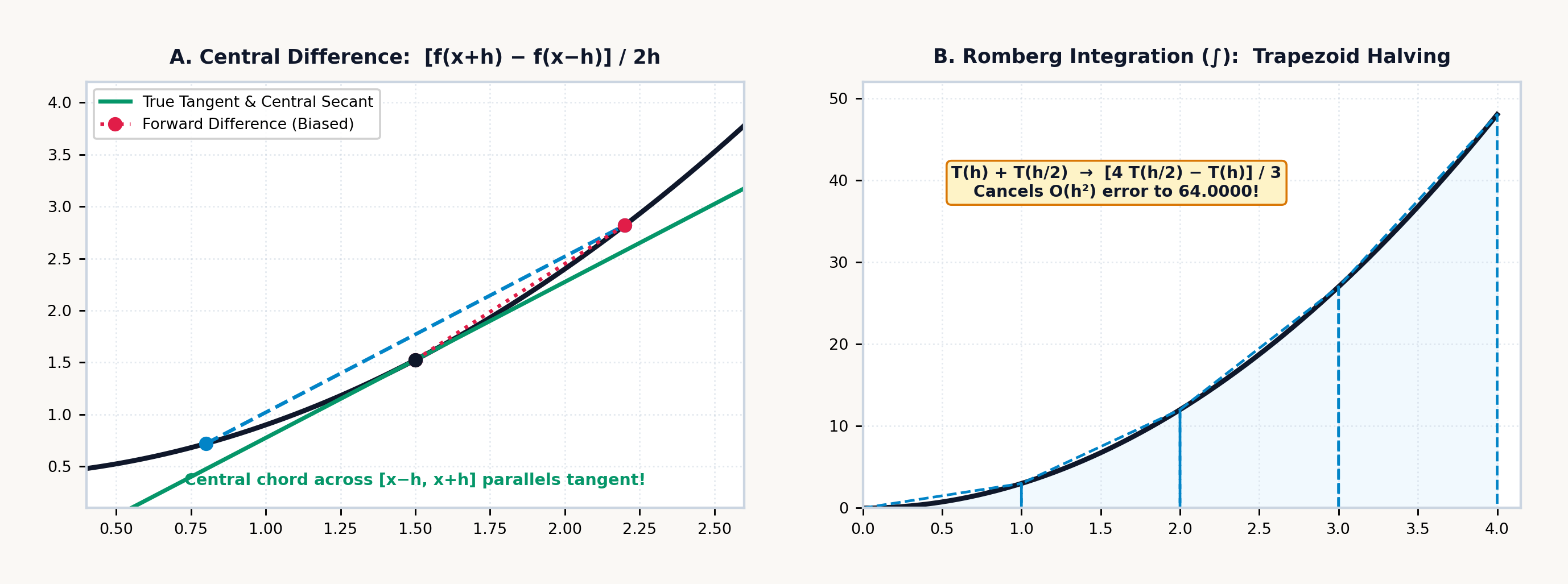
The leading \(h^2\) error cancels to zero. Across a single coarse macro-panel of span \(h = b - a\) (subdivided into two sub-steps of width \(h/2\) at the midpoint \(m = \frac{a+b}{2}\)), substituting \(T(h) = \frac{h}{2}[f(a) + f(b)]\) and \(T(h/2) = \frac{h}{4}[f(a) + 2f(m) + f(b)]\) into Richardson's \(\frac{4}{3} - \frac{1}{3}\) combination yields:
Those \(1\text{–}4\text{–}1\) weights \(\frac{h}{6}[f(a) + 4f(m) + f(b)]\) (with \(h = b - a\), or \(\frac{\Delta x}{3}\) in terms of the half-step \(\Delta x = h/2\)) show that Richardson's \(\frac{4}{3} - \frac{1}{3}\) combination of two flat-topped trapezoid sums produces Simpson's Parabolic Rule (\(\mathcal{O}(h^4)\)), the exact area under a parabola fitted through the left endpoint, the midpoint, and the right endpoint. Because the third derivative \(f'''(x)\) of any cubic polynomial \(Ax^3 + Bx^2 + Cx + D\) is a constant (so \(f'''(b) - f'''(a) = 0\) in the \(h^2\) term and \(f^{(4)}(x) = 0\) in the \(h^4\) term), Simpson's \(1\text{–}4\text{–}1\) rule is exact for both parabolas and cubics: on \(\int_0^4 x^3\,dx = \left[\frac{1}{4}x^4\right]_0^4 = \mathbf{64}\), while the single trapezoid \(T(4) = 128\) overshoots by \(100\%\) and the two-panel trapezoid \(T(2) = 80\) overshoots by \(25\%\), combining them via \(\frac{4 T(2) - T(4)}{3}\) produces the exact value \(\mathbf{64}\).
8.2.3 Werner Romberg's Triangular Tableau
In 1955, Werner Romberg (Romberg, 1955) extended Richardson's elimination beyond the \(h^2\) term. Once two Simpson parabolic estimates are available at step sizes \(h\) and \(h/2\) across a macro-panel of span \(h = b - a\) (subdivided into four sub-steps of width \(h/4\) at nodes \(x_0, x_1, x_2, x_3, x_4\)), their leading \(c_2 h^4\) errors stand in the ratio \(\left(\frac{1}{2}\right)^4 = \frac{1}{16}\).
The combination \(\frac{16}{15}S_{\text{fine}} - \frac{1}{15}S_{\text{coarse}}\) eliminates the \(h^4\) error and produces Boole's 5-Point Rule (\(\mathcal{O}(h^6)\)) with its \(7\text{–}32\text{–}12\text{–}32\text{–}7\) weights (where \(\frac{h}{90} = \frac{2(h/4)}{45}\)):
Organizing these successive step-halvings into a lower-triangular array \(R(k, j)\) indexed by row \(k\) (where row \(k\) partitions \([a, b]\) into \(2^k\) panels of width \(h_k = (b-a)/2^k\)) and extrapolation column \(j\) (where each column \(j \ge 1\) cancels the \(h^{2j}\) error term from column \(j - 1\)) defines Romberg Integration (Romberg, 1955):
Each extrapolated entry \(R(k, j)\) takes the fine-grid estimate \(R(k, j-1)\) immediately to its left and adds the fraction \(\frac{1}{4^j - 1}\) of its improvement \(R(k, j-1) - R(k-1, j-1)\) over the coarser row \(R(k-1, j-1)\) directly above it. Across each row of the tableau, the base column \(j = 0\) accumulates the midpoint-reusing trapezoidal sum \(T(h_k)\) at \(\mathcal{O}(h^2)\), while successive columns apply the multipliers \(\frac{4 R(k,0) - R(k-1,0)}{3}\) (\(j = 1\), Simpson's \(\mathcal{O}(h^4)\) rule), \(\frac{16 R(k,1) - R(k-1,1)}{15}\) (\(j = 2\), Boole's \(\mathcal{O}(h^6)\) rule), and \(\frac{64 R(k,2) - R(k-1,2)}{63}\) (\(j = 3\), 9-point \(\mathcal{O}(h^8)\) extrapolation), up to the capped high-order limit \(j_{\max} = 5\) (\(\mathcal{O}(h^{12})\)). On \(\int_0^2 e^x\,dx = e^2 - 1 \approx \mathbf{6.389}\), the first four rows of \(R(k, j)\) feed each successive column to the right:
| Row \(k\) (Panels \(2^k\)) | \(j = 0\) (Trapezoid \(\mathcal{O}(h^2)\)) | \(j = 1\) (Simpson \(\mathcal{O}(h^4)\)) | \(j = 2\) (Boole \(\mathcal{O}(h^6)\)) | \(j = 3\) (\(\mathcal{O}(h^8)\)) |
|---|---|---|---|---|
| \(k = 0\) (\(1\) panel) | \(8.389\) | — | — | — |
| \(k = 1\) (\(2\) panels) | \(6.913\) | \(6.421\) | — | — |
| \(k = 2\) (\(4\) panels) | \(6.522\) | \(6.391\) | \(6.389\) | — |
| \(k = 3\) (\(8\) panels) | \(6.422\) | \(6.389\) | \(6.389\) | \(6.389\) |
On Row \(k = 0\) (\(1\) trapezoid, \(h_0 = 2\)), the single trapezoid \(R(0,0) = \frac{2}{2}(e^0 + e^2) \approx 8.389\) overshoots the exact integral by \(+31.3\%\). On Row \(k = 1\) (\(2\) trapezoids, \(h_1 = 1\)), adding the single midpoint \(e^1\) gives \(R(1,0) \approx 6.913\), and applying \(\frac{4 R(1,0) - R(0,0)}{3}\) produces the Simpson estimate \(R(1,1) \approx 6.421\), which reduces the error tenfold. On Row \(k = 2\) (\(4\) trapezoids, \(h_2 = 0.5\)), adding the two quarter-points gives \(R(2,0) \approx 6.522\), which extrapolates to \(R(2,1) \approx 6.391\) and then \(R(2,2) = \frac{16 R(2,1) - R(1,1)}{15} \approx 6.389\), within \(0.003\%\) of the exact value using only \(5\) function evaluations. By Row \(k = 3\) (\(8\) trapezoids, \(h_3 = 0.25\)), using \(9\) function evaluations, \(R(3,3) \approx 6.389\) is accurate to seven significant digits, and by Row \(k = 4\) (\(17\) points), the error drops below \(10^{-12}\).
Both the logarithmic benchmark \(\int_1^2 \frac{1}{x}\,dx = \ln 2 \approx \mathbf{0.693}\) and the exponential decay benchmark \(\int_0^1 e^{-x}\,dx = 1 - e^{-1} \approx \mathbf{0.632}\) show this rapid contraction across the first two Romberg rows: for \(\int_1^2 \frac{1}{x}\,dx\), the single trapezoid \(R(0,0) = \frac{1}{2}(1 + \frac{1}{2}) = 0.75\) and two-panel trapezoid \(R(1,0) = \frac{1}{2}(0.75) + \frac{1}{2}(\frac{2}{3}) \approx 0.708\) combine via \(\frac{4 R(1,0) - R(0,0)}{3}\) to yield \(R(1,1) \approx \mathbf{0.694}\), and one more halving to \(R(2,2)\) reaches \(\approx \mathbf{0.693}\).
The Romberg tableau caps extrapolation at column \(j_{\max} = 5\) (\(\mathcal{O}(h^{12})\)) because fitting an unbounded polynomial degree across equally spaced points on a wide interval triggers violent oscillations near the boundaries (Runge's Phenomenon); capping the extrapolation order at \(j_{\max} = 5\) and splitting wide domains across logarithmic \(1\text{–}2\text{–}5\) decade boundaries prevents high-degree ringing. When an integrand is a periodic wave (such as \(\cos^2 x\)) or a bell curve whose odd derivatives \(f^{(2m-1)}(b) - f^{(2m-1)}(a)\) vanish at both endpoints in the Euler–Maclaurin expansion, the Composite Trapezoidal Rule converges exponentially fast on its own. Comparing adjacent high-order Romberg entries \(|R(k, j) - R(k, j-1)|\) (and \(|R(k, j) - R(k-1, j-1)|\) along the diagonal) also provides a self-contained truncation error estimate \(\pm\varepsilon\) that is returned in Register \(Y\) alongside the converged integral \(I\) in Register \(X\).
8.2.4 Endpoint-Clustering Transforms & Singularity Substitutions
Physical integrals routinely span an infinite upper limit \([a, \infty)\) or involve an integrand whose value or slope diverges at an endpoint—such as an inverse-square-root pendulum turnaround cusp \(\int_0^b \frac{g(x)}{\sqrt{x}}\,dx\) or the square-root boundary ribbon \((H - y)\sqrt{8y}\) at \(y = 0\) of a parabolic arch. If a closed trapezoidal rule evaluates an endpoint that triggers a division by zero (such as \(\frac{\sin x}{x}\) at \(x = 0\) or \(\frac{1}{\sqrt{1 - u^2}}\) at \(u = \pm 1\)), the unguarded evaluation halts at the pole.
To protect Romberg quadrature against integrable endpoint singularities and to accelerate Euler–Maclaurin convergence, a cubic polynomial change of variable (Kahan, 1979) can be applied after normalizing the integration interval \([a, b]\) onto the standard symmetric domain \(u \in [-1, 1]\) via the affine linear map \(x(u) = \frac{a + b}{2} + \frac{b - a}{2}u\). Like a surveyor approaching the crumbly rim of a canyon who takes progressively shorter steps near the edge and stops just short of the precipice, the S-shaped cubic curve \(u(t) = \frac{1}{2}t(3 - t^2)\) crowds sample points densely toward the boundaries \(u = \pm 1\) while its slope \(\frac{du}{dt} = \frac{3}{2}(1 - t^2)\) tapers smoothly to zero right at the endpoints:
Under this change of variable, the normalized integral \(\int_{-1}^{1} \tilde{f}(u)\,du\) becomes:
This cubic mapping accomplishes three numerical objectives at once. First, it suppresses endpoint singularities via the \((1 - t^2)\) Jacobian factor (the chain-rule stretching factor \(\frac{du}{dt} = \frac{3}{2}(1 - t^2)\)): at both ends of the interval (\(t = \pm 1\)), the transformation maps \(u(\pm 1) = \pm\frac{1}{2}(3 - 1) = \pm 1\) while its first derivative \(\frac{du}{dt} = \frac{3}{2}(1 - t^2)\) vanishes (\(\frac{du}{dt}\big|_{t=\pm 1} = 0\)). Multiplying the integrand by the vanishing weight \(\frac{3}{2}(1 - t^2)\) forces the transformed integrand to zero at \(t = \pm 1\) for any bounded function (so the endpoints \(u = \pm 1\) never need to be sampled at all) and softens an integrable \(1/\sqrt{1 - u^2}\) singularity because \(1 - u^2 = \frac{1}{4}(1 - t^2)^2(4 - t^2)\) shares a double factor of \((1 - t^2)\).
Second, the cubic change of variable ensures vanishing odd Euler–Maclaurin endpoint derivatives: because the Euler–Maclaurin error series \(\sum \frac{B_{2m}}{(2m)!}h^{2m}[g^{(2m-1)}(1) - g^{(2m-1)}(-1)]\) is driven by the odd-order derivatives at the endpoints, and the chain rule multiplies the first derivative of \(g(t) = \tilde{f}(u(t))\frac{3}{2}(1 - t^2)\) by \((1 - t^2)\), the leading \(h^2\) endpoint error term is annihilated even before Richardson extrapolation begins. Third, it creates dense node clustering near the boundaries: uniformly spaced Romberg steps \(t_i\) in \([-1, 1]\) map through \(u(t) = \frac{1}{2}t(3 - t^2)\) into non-uniformly clustered nodes \(u_i\) that crowd densely toward \(u = \pm 1\) where boundary layers and square-root tangents vary fastest, mapping the halfway node \(t = 0.5\) to \(u(0.5) \approx \mathbf{0.688}\) with Jacobian weight \(w(0.5) = \mathbf{1.125}\), and clustering the three-quarter node \(t = 0.75\) to \(u(0.75) \approx \mathbf{0.914}\) while the weight tapers smoothly to \(w(0.75) \approx \mathbf{0.656}\).
Whereas open-quadrature integrators apply the cubic transformation \(u(t) = \frac{1}{2}t(3 - t^2)\) internally, the SC-32 quadrature engine evaluates closed composite trapezoidal panels with adaptive sub-panel refinement, so a removable or integrable endpoint pole (such as \(t = 0\) in \(\frac{\sin t}{t}\)) is handled by displacing the limit to a nearby interior point like \(a = 10^{-12}\), while integrands whose value is finite at the endpoint—such as \((4 - y)\sqrt{8y} = 0\) at \(y = 0\), where only the derivative \(y^{-1/2}\) diverges—integrate over \([0, 4]\) without displacement.
Alongside cubic endpoint clustering, two classical variable substitutions eliminate algebraic \(1/\sqrt{x}\) singularities and infinite \([a, \infty)\) tails analytically. First, whenever an integral has an integrable \(1/\sqrt{x}\) singularity at \(x = 0\) (as occurs when a pendulum reaches its turnaround point or light grazes a caustic), substituting \(x = u^2\) introduces the differential factor \(dx = 2u\,du\), canceling the singular root \(\sqrt{x} = u\):
The integrand of \(\int_0^1 \frac{\cos x}{\sqrt{x}}\,dx\) diverges to \(+\infty\) at \(x = 0\), yet the smooth transformed integrand \(2\cos(u^2)\) over \([0, 1]\) converges in four Romberg rows to \(\approx \mathbf{1.809}\). Second, when integrating a rapidly decaying tail over \([a, \infty)\) with \(a > 0\), the reciprocal substitution \(x = 1/t\) (\(dx = -dt/t^2\)) maps the infinite horizon \(x \to \infty\) onto the finite interval \([0, 1/a]\) as \(t \to 0^+\):
A small shift of the lower limit from \(0\) to \(10^{-12}\) (or truncating a Gaussian or exponential tail at \(5\) to \(8\) characteristic scale lengths where \(e^{-x^2/2}\) has already fallen below machine epsilon) lets Romberg's tableau integrate improper tails to full precision.
8.2.5 Non-Elementary Integrals in Probability, Mechanics & Blackbody Radiation
Introductory calculus courses construct nearly every exercise so that a closed-form symbolic antiderivative \(F(x)\) exists for evaluating \(F(b) - F(a)\). While any elementary combination of powers, roots, sines, exponentials, and logarithms can be differentiated by direct analytical rules, most continuous curves encountered in physics possess no elementary antiderivative and require Romberg quadrature.
In astronautics, the ideal rocket equation integrates the momentum balance \(m\frac{dv}{dt} = -v_e\frac{dm}{dt} - mg(h)\sin\gamma\) of a launch vehicle expelling propellant at effective exhaust speed \(v_e = I_{\text{sp}} g_0\). In vacuum with zero gravity loss, separating variables yields the logarithmic velocity increment \(\Delta v_{\text{ideal}} = \int_{m_f}^{m_0} \frac{v_e}{m}\,dm = I_{\text{sp}} g_0 \ln\!\left(\frac{m_0}{m_f}\right)\). When atmospheric drag \(D(v, h(t))\) and altitude-dependent gravity \(g(h(t))\) act together during ascent, however, the net acceleration \(a(t) = \frac{F_{\text{thrust}}(t) - D(t)}{m_0 - \dot{m}t} - g(t)\sin\gamma(t)\) cannot be integrated in closed form and requires numerical quadrature \(\Delta v = \int_0^{t_b} a(t)\,dt\).
A simple pendulum of length \(L\) under gravity \(g\) has the small-angle period \(T_0 = 2\pi\sqrt{L/g}\), which assumes that the restoring pull of gravity grows linearly with angle \(\theta\). A real pendulum swinging through a wide release angle \(\theta_0\), however, runs noticeably slower than \(T_0\): as the bob swings out toward the horizontal, gravity's true tangential restoring pull \(\sin\theta = \theta - \theta^3/6 + \dots\) falls below the linear spring approximation \(\theta\), so the bob lingers longer near its turnaround points. Retaining the exact restoring torque \(\sin\theta\) in conservation of energy and parameterizing the quarter-swing from bottom dead center (\(\varphi = 0\)) to peak release (\(\varphi = \pi/2\)) by the normalized phase angle \(\varphi \in [0, \pi/2]\) (defined via \(\sin(\theta/2) = k\sin\varphi\), with amplitude modulus \(k = \sin(\theta_0/2)\)) leads to the Complete Elliptic Integral of the First Kind \(K(k)\):
Because \(\sqrt{1 - k^2\sin^2\varphi}\) tracks the bob's angular speed at phase \(\varphi\), a tiny swing (\(k \to 0\)) reduces the integrand to \(1\) and recovers the small-angle limit \(T(\theta_0)/T_0 = 1\), whereas a wider release (\(k > 0\)) depresses \(\sqrt{1 - k^2\sin^2\varphi}\) below \(1\) and stretches the time the bob spends lingering near its turnaround peak \(\varphi = \pi/2\). Like the perimeter of an ellipse, no finite combination of elementary functions can express \(K(k)\), yet Romberg quadrature evaluates it to twelve digits—and \(2/\pi\,K(k)\) also equals the reciprocal of the Arithmetic-Geometric Mean \(\operatorname{AGM}(1, \cos(\theta_0/2))\). For a pendulum released at \(\theta_0 = 60^\circ\) (\(k = \sin 30^\circ = 0.5\), \(\cos 30^\circ = \frac{\sqrt{3}}{2} \approx 0.866\)), integrating \((1 - 0.25\sin^2\varphi)^{-1/2}\) over \([0, \pi/2]\) and scaling by \(2/\pi\) (or running two steps of the AGM recurrence \(a_{n+1} = \frac{a_n+b_n}{2},\; b_{n+1} = \sqrt{a_n b_n}\)) yields \(\frac{T(60^\circ)}{T_0} \approx \mathbf{1.073}\), meaning the clock runs \(\approx \mathbf{7.318\%}\) slower than the small-angle formula.
Non-elementary integrals also govern normal probability, quantum thermal radiation, and solid-state heat capacity. The Gaussian normal error integral \(\frac{1}{\sqrt{2\pi}}\int_a^b e^{-x^2/2}\,dx\) has no closed-form antiderivative in elementary functions, requiring numerical quadrature across finite confidence intervals. In thermal physics, light of wavelength \(\lambda\) and frequency \(\nu = c/\lambda\) (traveling at the speed of light \(c\)) is emitted in discrete energy quanta \(E = h\nu = hc/\lambda\) governed by Planck's constant \(h \approx 6.626 \times 10^{-34}\text{ J}\cdot\text{s}\), while a cavity at absolute temperature \(T\) supplies thermal agitation energy \(k_B T\) per degree of freedom via Boltzmann's constant \(k_B \approx 1.381 \times 10^{-23}\text{ J/K}\).
Comparing photon energy \(hc/\lambda\) against thermal energy \(k_B T\) defines the dimensionless photon-energy ratio \(x = \frac{hc}{\lambda k_B T} = \frac{h\nu}{k_B T}\) and yields Planck's blackbody spectral radiance law \(B_\lambda(\lambda, T) \propto \lambda^{-5}/(e^{hc/\lambda k_B T} - 1)\). Integrating Planck's distribution over the entire spectrum \(x \in [0, \infty)\) collapses via the zeta identity \(\int_0^\infty \frac{x^3}{e^x - 1}\,dx = \frac{\pi^4}{15} \approx 6.494\) into the Stefan–Boltzmann \(T^4\) total radiation law. When an astronomer or optical engineer asks how much thermal power a star or furnace emits inside a finite detector wavelength band \([\lambda_1, \lambda_2]\) (corresponding to \([x_1, x_2]\)), however, no closed-form antiderivative exists for \(\int_{x_1}^{x_2} \frac{x^3}{e^x - 1}\,dx\) (which weights the cubic electromagnetic mode density and photon energy \(x^3\) by the Bose–Einstein thermal occupancy factor \(\frac{1}{e^x - 1}\)).
A companion quantum integral governs the Debye model of solid heat capacity. Classical physics predicted that every crystal lattice should have a constant molar heat capacity of \(3R\) (the Dulong–Petit ceiling, where \(R = N_A k_B \approx 8.314\text{ J/(mol}\cdot\text{K)}\) is the molar gas constant), yet experiments showed that the molar heat capacity \(C_V(T)\) of diamond or copper drops toward zero as \(T^3\) at cryogenic temperatures. Peter Debye explained this drop by modeling atomic lattice vibrations as acoustic phonons up to a crystal-specific cutoff frequency \(\nu_D\), which defines the Debye temperature \(\Theta_D = h\nu_D / k_B\). Integrating the temperature derivative of the Bose–Einstein phonon energy across the dimensionless phonon energy \(x = \frac{h\nu}{k_B T}\) from \(0\) to the upper cutoff \(\Theta_D / T\) gives the Debye heat-capacity integral:
The cubic prefactor \(\left(\frac{T}{\Theta_D}\right)^3\) measures the fraction of the crystal's vibrational spectrum that is thermally active at temperature \(T\), while the integrand pairs \(x^4\)—combining the quadratic acoustic mode density (\(\propto x^2\)) with the squared phonon energy (\(\propto x^2\))—against the Bose–Einstein temperature derivative \(\frac{e^x}{(e^x - 1)^2}\), showing how high-frequency lattice modes (\(h\nu \gg k_B T\), or \(x \gg 1\)) "freeze out" exponentially when thermal energy \(k_B T\) is too small to excite them. In the cryogenic limit \(T \ll \Theta_D\), where the upper limit \(\Theta_D / T \to \infty\), \(\int_0^\infty \frac{x^4 e^x}{(e^x - 1)^2}\,dx = \frac{4\pi^4}{15} \approx 25.976\) yields the Debye \(T^3\) Law \(C_V(T) = \frac{12\pi^4}{5} R \left(\frac{T}{\Theta_D}\right)^3\) (giving \(C_V \approx \mathbf{0.753\text{ J/(mol}\cdot\text{K)}}\) for copper with \(\Theta_D = 343\text{ K}\) at \(T = 25\text{ K}\)); at intermediate temperatures (such as \(T = 171.5\text{ K}\), where \(\Theta_D / T = 2\)), Romberg quadrature evaluates \(\int_0^2 \frac{x^4 e^x}{(e^x - 1)^2}\,dx \approx \mathbf{2.201}\).
Across physical optics and civil highway design, when coherent light grazes a sharp edge—or when an engineer lays out a highway exit ramp connecting a straight tangent road (\(\kappa = 0\)) to a circular curve—the transition path must avoid a sudden jump in centrifugal force. If a driver turns the steering wheel at a constant rate as normalized arc distance \(t\) advances from \(0\) to \(u\), the road's curvature grows linearly with distance as \(\kappa(t) = \pi t\). Because the vehicle's compass heading angle \(\theta(t)\) is the cumulative integral of curvature along the path (\(\theta(t) = \int_0^t \pi s\,ds = \frac{\pi}{2}t^2\)), the heading angle grows with the square of arc distance \(t\), and integrating the horizontal component \(\cos\theta(t)\) and lateral component \(\sin\theta(t)\) yields the Fresnel Diffraction Integrals—tracing the double-coiled clothoid spiral \((C(u), S(u))\):
The quadratic phase \(\frac{\pi t^2}{2}\) inside the cosine and sine reflects the linearly tightening curvature, and the leading Taylor terms show that for small arc distances \(u\), the ramp advances forward almost linearly (\(C(u) \approx u\)) while deflecting sideways as the cube of distance (\(S(u) \approx \frac{\pi}{6}u^3\)). For a clothoid highway transition spiral at normalized arc parameter \(u = 0.6\), integrating \(\cos(\pi t^2/2)\) and \(\sin(\pi t^2/2)\) yields the horizontal and lateral clothoid coordinates \((C(0.6), S(0.6)) \approx (\mathbf{0.581},\; \mathbf{0.111})\).
In clinical pharmacology and bioequivalence trials, when a patient swallows an oral dose \(D\) of a medication with bioavailability fraction \(F \in (0, 1]\) (the fraction of the dose that reaches systemic circulation), the absorbed drug disperses across an apparent volume of distribution \(V_d\) (the effective fluid volume of blood and tissue into which the drug dilutes). Two competing first-order rate constants govern the bloodstream concentration \(C(t)\) over time \(t\): rapid absorption from the gut into the blood at rate \(k_a\), and slower clearance by the liver and kidneys at elimination rate \(k_e\) (\(k_a > k_e\)), combining into the Bateman bi-exponential equation:
The concentration scale \(A = \frac{F D k_a}{V_d(k_a - k_e)}\) normalizes the absorbed dose \(FD\) by the distribution volume \(V_d\) and the relative speed of absorption over elimination, while the bi-exponential difference \((e^{-k_e t} - e^{-k_a t})\) shapes the rise-and-fall time profile: at \(t = 0\), both exponentials equal \(1\) so plasma concentration starts at \(1 - 1 = 0\); as the faster gut-absorption term \(e^{-k_a t}\) decays toward zero, \(C(t)\) climbs to a peak at \(t_{\max} = \frac{\ln(k_a / k_e)}{k_a - k_e}\) (where \(C'(t_{\max}) = 0\)); and once absorption is complete, the slower elimination exponential \(e^{-k_e t}\) governs the long terminal decay tail. Total systemic drug exposure is measured by the definite integral of plasma concentration over time—the Area Under the Plasma Concentration–Time Curve (\(\text{AUC}\)), which determines the patient's apparent oral clearance \(\text{CL}/F\) (the volume of blood cleared of drug per hour):
Total lifetime exposure \(\text{AUC}_{0\to\infty} = \text{AUC}_{0\to T} + \text{AUC}_{T\to\infty}\) combines the measured integral \(\text{AUC}_{0\to T}\) up to the final blood sample at time \(T\) (typically \(T = 24\text{ hr}\), after the rapid absorption term \(e^{-k_a T}\) has died out) with the single-exponential terminal tail \(\text{AUC}_{T\to\infty} \approx C(T)/k_e\) from \(T\) to \(\infty\) (where \(k_e = \frac{\ln 2}{t_{1/2}}\)), so dividing the administered \(\text{Dose}\) by \(\text{AUC}_{0\to\infty}\) yields the apparent oral clearance \(\text{CL}/F\) in \(\text{L/hr}\).
8.3 Numerical Calculus in Four Registers
Central-difference differentiation and adaptive Romberg quadrature on the SC-32 map their two-point interval geometry onto Registers \(Y\) and \(X\) while leaving Registers \(Z\) and \(T\) undisturbed for multi-integral chaining:
- Storing & Selecting the Integrand (
[↱] [EQN],SCRL, andFN=): Press[↱] [EQN](right-shifted on[STO]), tap the first top-row softkey (NEW), press a letter key (A–Z) to label the slot, enter the RPN integrand expression using[RCL]+ letter for the variable of integration (insertingLBL/RTNtokens on[+]if needed and using right-shiftedSCRLon[RCL]to scroll long formulas), and press[↱] [EQN]again to save the equation and return to the stack, or pre-select an existing equation withFN=(left-shifted on[XEQ]). (When integrating trigonometric functions, ensure radian mode is active via[↰] [MODES]\(\to\)RAD.) - Staging Limits \([a, b]\) Across \((Y, X)\): Type the lower limit \(a\), press
[ENTER], and type the upper limit \(b\) so the integration interval sits across Register \(Y = a\) and Register \(X = b\). If \(a = b\), the integrator returns \(0\); if \(b < a\), it preserves the orientation identity \(\int_a^b f(x)\,dx = -\int_b^a f(x)\,dx\) by reversing the sign. - Selecting the Equation & Dummy Variable (
[↱] [∫]Softkeys): Press[↱] [∫](right-shifted on[8]). The top-row softkeys list your stored equations ([A],[B], etc., or you can press the equation's letter key); tapping the equation's softkey prompts∫ _in Alpha mode to press or tap the dummy variable of integration (X,T,R, orV; typing a value + tapping a variable softkey stores that parameter directly). If the integrand references any extra parameter variable not already stored, the calculator prompts (A?,B?\(\to\) type value +[ENTER]or[XEQ]) before integrating. - Reading the Post-Integration Audit Frame (
Y = ±ε,X = I): Following William Kahan's display-coupled stopping rule (Kahan, 1979; HP, 1982; HP, 1991), the convergence tolerance scales with the active[↰] [DISP]setting (FIX,SCI,ENG, orALL) while keeping internal sums in full 64-bit precision. Upon convergence, the calculator replaces \((Y, X)\) in place with the certified definite integral \(I = \int_a^b f(x)\,dx\) in Register \(X\) and the estimated Richardson truncation uncertainty \(\pm\varepsilon\) in Register \(Y\), leaving Registers \(Z\) and \(T\) untouched for multi-integral chaining.
8.3.1 Algebraic Integrands & Boundary Cusps
Unless degree mode is specified, trigonometric and calculus sequences use radian measure. On the stack, Richardson's single-step error cancellation \(R(1,1) = T(h/2) + \frac{T(h/2) - T(h)}{3}\) combines any coarse estimate \(T(h)\) in Register \(Y\) and fine estimate \(T(h/2)\) in Register \(X\) by duplicating \(T(h/2)\), subtracting \(T(h)\), dividing by \(3\), and adding back to \(T(h/2)\), while the built-in Romberg integrator consumes only the limits \((a, b)\) in Registers \(Y\) and \(X\) and returns \((\pm\varepsilon, I)\) in place without disturbing Registers \(Z\) and \(T\).
In mechanical and electromagnetic accumulation laws, the analytical smoothness of the integrand governs which column of Romberg's tableau delivers the final answer. Because Richardson's first \(\frac{4}{3} T(h/2) - \frac{1}{3} T(h)\) column \(R(1,1)\) is algebraically identical to Thomas Simpson's parabolic rule—whose fourth-order error \(\propto f^{(4)}(\xi)\,h^4\) vanishes for every polynomial of degree \(3\) or less—any cubic velocity, force, or energy law hits machine precision on the very first Romberg row. If a solid-propellant sounding rocket climbs at \(v(t) = 30t - 0.5t^3\text{ m/s}\) over \(t \in [0, 6]\text{ s}\), one Simpson pass integrates the burnout altitude \(\int_0^6 (30t - 0.5t^3)\,dt = [15t^2 - \frac{1}{8}t^4]_0^6 = \mathbf{378\text{ m}}\) in Register \(X\) (\(\pm\varepsilon = 0\) in Register \(Y\)); a liquid-bipropellant upper stage accelerating exponentially as \(a(t) = 12e^{0.04t} - 9.807\text{ m/s}^2\) over a \(25\text{-second}\) burn integrates over \([0, 25]\) across higher Romberg columns to \(\Delta v \approx \mathbf{270.31\text{ m/s}}\).
Simpson's exactness on cubics also governs the variable-pitch progressive suspension spring (\(F(x) = 2500x + 40000x^3\text{ N}\)) of an off-road rally car and the voltage-dependent capacitance of a nonlinear ceramic capacitor. Over small road ripples (\(x \ll 0.05\text{ m}\)), the \(2,500\text{ N/m}\) linear spring rate gives a supple ride; on hard jump landings, the lower coils bind so the \(40,000x^3\) stiffening prevents bottoming out, and integrating \(F(x)\) over \([0, 0.15]\text{ m}\) converges on the first Simpson column to \(W = [1250x^2 + 10000x^4]_0^{0.15} \approx 28.125 + 5.063 \approx \mathbf{33.188\text{ Joules}}\) (\(18\%\) above a linear spring's \(28.125\text{ J}\)). For a Class-II barium titanate (\(\text{BaTiO}_3\)) ceramic capacitor whose capacitance droops under high DC bias as \(C(V) = C_0(1 - \alpha V^2)\) with \(C_0 = 10\,\mu\text{F}\) and \(\alpha = 10^{-6}\text{ V}^{-2}\) (Horowitz & Hill, 2015), integrating the differential energy \(dW = C(V)V\,dV = 10^{-5}(V - 10^{-6}V^3)\,dV\) over \([0, 500]\text{ V}\) is again a degree-3 polynomial that Simpson's column \(R(1,1)\) resolves to \(\approx \mathbf{1.094\text{ Joules}}\)—a \(12.5\%\) saturation shortfall below the unadjusted linear estimate \(\frac{1}{2}C_0 V^2 = 1.25\text{ J}\).
Unlike those cubic polynomials, a parabolic arch load ribbon \((H - y)\sqrt{8y}\) of width \(w(y) = \sqrt{8y}\text{ m}\) and height \(H = 4\text{ m}\) (scaled by \(9,810\text{ N/m}^3\)) has a vertical tangent at the arch base \(y = 0\), where its derivative \(\frac{d}{dy}\sqrt{8y} = \frac{\sqrt{2}}{\sqrt{y}} \to \infty\) diverges. Because \((4 - y)\sqrt{8y}\) evaluates to a finite \(0\) at \(y = 0\) even though its derivative \(d/dy(\sqrt{8y}) \propto y^{-1/2}\) has a vertical tangent there, Romberg extrapolation across \([0, 4]\) refines the endpoint panel across higher Romberg columns \(R(k, j)\) to full precision, converging to \(F = \frac{4}{15}(9810)\sqrt{8}\,H^{5/2} \approx \mathbf{236,773.292\text{ N}}\) within \(10^{-3}\text{ N}\) of exact \(236,773.291\text{ N}\) (with first moment \(M_0 = \frac{8}{105}(9810)\sqrt{8}\,H^{7/2} \approx \mathbf{270,598.047\text{ N}\cdot\text{m}}\) and centroid height \(y_{\text{cp}} = M_0 / F = \frac{2}{7}H \approx \mathbf{1.143\text{ m}}\)).
8.3.2 Transcendental Integrals, Piecewise RMS Waveforms & Chained Centroids
On Gaussian bells, pharmacokinetic clearance curves, Planck blackbody bands, and chained integral ratios, Euler–Maclaurin endpoint behavior and four-register stack preservation govern both accuracy and register allocation. For the non-elementary standard normal density \(\phi(x) = \frac{1}{\sqrt{2\pi}}e^{-x^2/2}\), truncating the lower \((-\infty, 0]\) tail at five standard deviations (\(x = -5\), where \(\phi(-5) \approx 1.487 \times 10^{-6}\)) pairs an exponentially small left endpoint with the symmetry peak \(x = 0\), where every odd derivative \(\phi'(0) = \phi'''(0) = \phi^{(5)}(0) = 0\) vanishes; integrating across \([-5, 0]\) converges rapidly to \(\approx \mathbf{0.5}\) in Register \(X\) (\(\pm\varepsilon \approx 2.15 \times 10^{-10}\) in Register \(Y\)), missing only the minuscule five-sigma cumulative normal tail \(\Phi(-5) \approx 2.867 \times 10^{-7}\).
In clinical pharmacokinetics, an oral antibiotic regimen (\(\text{Dose} = 500\text{ mg}\), \(A = 25\text{ mg/L}\), \(k_a = 1.2\text{ hr}^{-1}\), \(k_e = 0.2\text{ hr}^{-1}\), peaking at \(t_{\max} = \frac{\ln(1.2/0.2)}{1.2 - 0.2} = \ln(6) \approx \mathbf{1.792\text{ hr}}\)) follows Bateman's bi-exponential curve \(25(e^{-0.2t} - e^{-1.2t})\). Integrating over \([0, 24\text{ hr}]\) gives the measured exposure \(\text{AUC}_{0\to 24} \approx \mathbf{103.138\text{ mg}\cdot\text{hr/L}}\) in Register \(X\); adding the analytically extrapolated terminal tail \(C(24)/k_e \approx 0.206 / 0.2 \approx 1.029\text{ mg}\cdot\text{hr/L}\) gives total systemic exposure \(\text{AUC}_{0\to\infty} \approx \mathbf{104.167\text{ mg}\cdot\text{hr/L}}\), and dividing into \(500\text{ mg}\) yields the apparent oral clearance \(\text{CL}/F \approx \mathbf{4.8\text{ L/hr}}\).
All four stack registers \((T, Z, Y, X)\) participate when chaining a Romberg integral into a subsequent normalization on the stack. To find the fraction of a blackbody's total Stefan–Boltzmann radiance emitted inside the dimensionless photon-energy band \([x_1, x_2] = [2, 6]\), integrating Max Planck's integrand \(x^3/(e^x - 1)\) over \([2, 6]\) places the band radiance integral \(I_{\text{band}} \approx \mathbf{4.41}\) in Register \(X\) and its Romberg uncertainty \(\approx 1.42 \times 10^{-11}\) in Register \(Y\); as we then form Euler's total radiation constant \(\pi^4 / 15 \approx \mathbf{6.494}\) in Register \(X\), the band integral \(\approx 4.41\) waits in Register \(Y\) while the uncertainty rides up into Registers \(Z\) and \(T\), so a single division and percentage scaling resolves \(\approx \mathbf{67.9\%}\).
On the True-RMS heating integral \(V_{\text{rms}} = \sqrt{\frac{1}{T}\int_0^T v(t)^2\,dt}\) for a pure sinusoid (\(\frac{1}{\pi}\int_0^\pi \sin^2 x\,dx = \mathbf{0.5}\)) versus a clipped AC waveform, any sharp slope corner must be split at the breakpoint before integrating. When a protection varistor clips a \(V_p = 170\text{ V}\) sine wave flat at \(V_c = 136\text{ V}\), the derivative \(v'(\theta)\) jumps discontinuously at the clipping knee \(\theta_c = \arcsin(136/170) = \arcsin(0.8) \approx 0.927\text{ rad}\), violating the smooth Euler-Maclaurin assumptions. Splitting the quarter-cycle \([0, \pi/2]\) right at \(\theta_c\) resolves the integral cleanly: first integrate the smooth rising sine squared \((170\sin\theta)^2\) over \([0, \theta_c]\) to obtain \(\approx 6,463.416\) in Register \(X\), then compute the flat clamped plateau \(136^2(\pi/2 - \theta_c) \approx 11,902.197\) while the rising-edge integral waits in Register \(Y\), sum to \(\approx 18,365.612\), multiply by \(2/\pi\), and take the square root to obtain the exact True-RMS voltage \(V_{\text{rms}} \approx \mathbf{108.129\text{ V}}\) without corner ringing.
Finally, when an engineering figure of merit is defined as the ratio of two definite integrals, the upper stack preserves the first integral without requiring a scratchpad variable. To find the optical mode confinement factor \(\Gamma = \int_{-d}^d |E(x)|^2\,dx / \int_{-5d}^{5d} |E(x)|^2\,dx\) of a double-heterostructure gallium arsenide \(\text{GaAs}/\text{AlGaAs}\) quantum-well laser diode—where only the central active layer \([-d, +d]\) stimulates emission while the evanescent wings in \([-5d, +5d]\) remain passive—model the transverse waveguide intensity profile in normalized half-width units \(d = 1\) as \(|E(x)|^2 = 1.23\,\operatorname{sech}^2(1.23\,x)\), evaluated via the reciprocal hyperbolic cosine \(1/\cosh(1.23\,x)\). Integrating first over the active core \([-1, 1]\) places \(I_{\text{core}} \approx \mathbf{1.685}\) in Register \(X\); typing the outer waveguide limits \([-5, 5]\) and integrating a second time lifts \(I_{\text{core}}\) into Register \(Z\) while placing the total mode energy \(I_{\text{total}} \approx \mathbf{2}\) in Register \(X\), so dropping the uncertainty and dividing core energy by total energy yields the optical confinement factor \(\Gamma \approx 1.685 / 2 \approx \mathbf{0.843}\) (\(\approx 84.3\%\)).
8.3.3 Central-Difference Derivatives & the Centrifugal Flyweight Governor
For numerical differentiation via the symmetric central-difference formulas \(f'(x_0) \approx \frac{f(x_0 + h) - f(x_0 - h)}{2h}\) and \(f''(x_0) \approx \frac{f(x_0 + h) - 2f(x_0) + f(x_0 - h)}{h^2}\), comparing the one-sided forward difference \(\frac{f(2 + 0.01) - f(2)}{0.01}\) against the symmetric central difference \(\frac{f(2 + 0.01) - f(2 - 0.01)}{0.02}\) on the cubic \(f(x) = x^3 - 2x\) at \(x_0 = 2\) (where the exact derivative is \(f'(2) = 3(2)^2 - 2 = \mathbf{10}\) and \(f''(2) = 12\)) eliminates the \(+\frac{1}{2}f''(2)h = +0.06\) parabolic bias while preserving the forward ordinate \(f(2.01) \approx 4.101\) across the upper registers:
| Keystroke | Register T | Register Z | Register Y | Register X | What Happens on the Stack |
|---|---|---|---|---|---|
2.01 [ENTER] 3 [yˣ] 2.01 [ENTER] 2 [×] [-] |
\(0\) | \(0\) | \(0\) | \(4.101\) | Evaluate forward ordinate \(f(2.01) = 2.01^3 - 2(2.01) \approx 4.101\) |
4 [-] 0.01 [÷] |
\(0\) | \(0\) | \(0\) | \(10.06\) | Forward difference \(D_{\text{fwd}}(0.01) \approx \mathbf{10.06}\) (\(+0.06\) bias) |
2.01 [ENTER] 3 [yˣ] 2.01 [ENTER] 2 [×] [-] |
\(10.06\) | \(10.06\) | \(10.06\) | \(4.101\) | Stage forward sample \(f(2.01) \approx 4.101\) |
1.99 [ENTER] 3 [yˣ] 1.99 [ENTER] 2 [×] [-] |
\(4.101\) | \(4.101\) | \(4.101\) | \(3.901\) | Stage backward sample \(f(1.99) \approx 3.901\) |
[-] 0.02 [÷] |
\(4.101\) | \(4.101\) | \(4.101\) | \(10\) | Central difference \(D_{\text{cen}}(0.01) \approx \mathbf{10}\) (\(600\times\) smaller error) |
On a quadratic parabola like \(f(x) = x^2\) at \(x_0 = 3\) using the \(\varepsilon_{\text{mach}}^{1/3}\) step size \(h = 10^{-5}\) (total span \(2h = 2 \times 10^{-5}\)), the \(+\frac{1}{2}f''(x_0)h^2 = 10^{-10}\) curvature terms on the right and left cancel to zero, returning the exact derivative \(\mathbf{6}\). On the exponential benchmark \(f(x) = e^{2x}\) at the origin \(x_0 = 0\) with step \(h = 10^{-5}\), evaluating \(\frac{e^{2h} - e^{-2h}}{2h} = 2\frac{\sinh(2h)}{2h}\) yields the first derivative \(f'(0) \approx \mathbf{2}\), while adding \(e^{2h} + e^{-2h} - 2 = 2(\cosh 2h - 1)\) and dividing by \(h^2 = 10^{-10}\) recovers the second derivative \(f''(0) \approx \mathbf{4}\).
Finally, evaluating the polar kinetic-energy equation \(E_k = \frac{1}{2}m\left(\dot{r}^2 + v_\theta^2\right)\) for a centrifugal flyball governor on a brass flyweight of mass \(m = 4\text{ kg}\) whirling at \(\omega = 40\text{ rad/s}\) along the cam slot \(r(\theta) = 0.15 + 0.05\sin(2\theta)\text{ m}\) at \(\theta = \pi/6\text{ rad}\) in radian mode pairs the radial and tangential velocity components across Register \(Y\) and Register \(X\): the radial slope \(\frac{dr}{d\theta} = 0.1\cos(\pi/3) = 0.05\text{ m/rad}\) (confirmed by the central difference \(\frac{r(\theta + 10^{-5}) - r(\theta - 10^{-5})}{2 \times 10^{-5}} = \mathbf{0.05\text{ m/rad}}\)) scales by \(\omega = 40\text{ rad/s}\) to give \(\dot{r}^2 = (2\text{ m/s})^2 = 4\text{ m}^2/\text{s}^2\) in Register \(Y\), while the tangential whirl speed \(v_\theta = 40\,r(\pi/6) \approx 40(0.193) \approx 7.732\text{ m/s}\) squares to \(\approx 59.785\text{ m}^2/\text{s}^2\) in Register \(X\), summing and scaling by \(\frac{1}{2}m = 2\text{ kg}\) to deliver the flyweight's kinetic energy \(E_k \approx \mathbf{127.569\text{ Joules}}\).
8.3.4 Practical Quadrature Strategy
When integrating complex physical waveforms on the stack, four numerical habits govern speed, accuracy, and boundary behavior. First, the active display format (FIX n, SCI n, ENG n) sets the relative convergence tolerance to \(10^{-\max(5,\, n+3)}\) (three orders of magnitude finer than the last displayed digit, down to \(10^{-11}\) in ALL), terminating once two successive horizontal extrapolations \(|R(k, j) - R(k, j-1)|\) (and diagonal steps \(|R(k, j) - R(k-1, j-1)|\)) satisfy this tolerance. Second, because post-integration leaves Registers \(Z\) and \(T\) undisturbed, typing new limits lifts the first integral \(I_1\) into Register \(Z\) (\(\approx 1.685\) in our laser confinement example) so \(I_1\) and \(I_2\) sit ready for immediate ratio or sum chaining.
Third, when an integrand contains a narrow spike (such as a high-\(Q\) resonance peak at \(x = 10\) inside \([0, 100]\)), splitting the interval at the peak (\([0, 10]\) and \([10, 100]\)) guarantees that the initial panel samples the apex. Fourth, for a removable \(0/0\) endpoint like the Sine Integral \(\operatorname{Si}(x) = \int_0^x \frac{\sin t}{t}\,dt = x - \frac{x^3}{3\cdot 3!} + \frac{x^5}{5\cdot 5!} - \dots\) (which governs Gibbs overshoot in Fourier square-wave synthesis and Fraunhofer slit diffraction), because closed Romberg quadrature samples both endpoints \(a\) and \(b\), evaluating \(\sin(0)/0\) at \(a = 0\) triggers DIVIDE BY 0, so displacing the lower limit to \(a = 10^{-12}\) integrates \(\operatorname{Si}(\pi) \approx 1.852\) and \(\operatorname{Si}(1) \approx \mathbf{0.946}\) without touching \(t = 0\), while \(x = u^2\) or \(x = 1/t\) substitutions tame \(1/\sqrt{x}\) cusps and semi-infinite tails.
8.3.5 Try It on the Stack
- Three-Point Simpson Check on a Quadratic Force Law: Evaluate the work \(W = \int_0^2 (3x^2 + 4x + 1)\,dx\) on the stack using Simpson's \((1, 4, 1)\frac{h}{6}\) rule with endpoints \(f(0) = 1\), midpoint \(f(1) = 8\), and upper limit \(f(2) = 21\) over span \(b - a = 2\). (Verified Register \(X\) result: \(W = \mathbf{18\text{ J}}\).)
- Symmetric Central-Difference Slope at \(x = 3\): For \(f(x) = x^3 - 2x\) at \(x_0 = 3\) with step \(h = 0.001\) (span \(2h = 0.002\)), evaluate \(\frac{f(3.001) - f(2.999)}{0.002}\) and compare against the exact analytical derivative \(f'(3) = 3(3^2) - 2\). (Verified Register \(X\) result: \(D_{\text{cen}} = \mathbf{25}\).)
- Near-Singular Sinc Ratio: In radian mode, evaluate \(\frac{\sin(0.003)}{0.003}\) by taking the sine of \(0.003\text{ rad}\) and dividing by \(0.003\) recalled via
LASTX, confirming the Maclaurin bound \(1 - x^2/6 = 1 - 1.5 \times 10^{-6}\). (Verified Register \(X\) result: \(\mathbf{\approx 1}\), differing from unity by \(1.5 \times 10^{-6}\).)