Chapter 7: Polynomial Evaluation, Cardano's Cubic & Brent's Root-Finder

In early 1535 in Venice and Milan, a public mathematical duel turned the inversion of equations into a high-stakes contest of livelihoods and honor (Cardano, 1545). Around 1515, Bologna mathematics professor Scipione del Ferro had discovered how to solve the "depressed" cubic \(t^3 + pt = q\) (a third-degree equation with no \(t^2\) term) and entrusted the manuscript on his deathbed in 1526 to his student Antonio Maria Fior. When Fior boasted that he alone could solve cubic equations, he challenged the Venetian mathematician Niccolò Fontana (Tartaglia): each contestant deposited thirty cubic problems with a notary and was given fifty days to solve the rival's list. On the night of February 12, 1535, eight days before the deadline, Tartaglia cracked the general reduction by dissecting a three-dimensional cube of side \((u - v)\) into smaller blocks, solving all thirty of Fior's problems within two hours while Fior failed to solve a single one of his.

Inverting a polynomial required a sixteenth-century breakthrough because, unlike forward arithmetic, running a physical design problem backward (where an unknown dimension, launch angle, or flow friction \(x\) must make a governing law balance to zero) places the unknown \(x\) in multiple incompatible powers at once, so no single division or root extraction can isolate it. On al-Khwarizmi's quadratic benchmark,

\[x^2 + 10x = 39 \tag{Eq. 7.1}\]

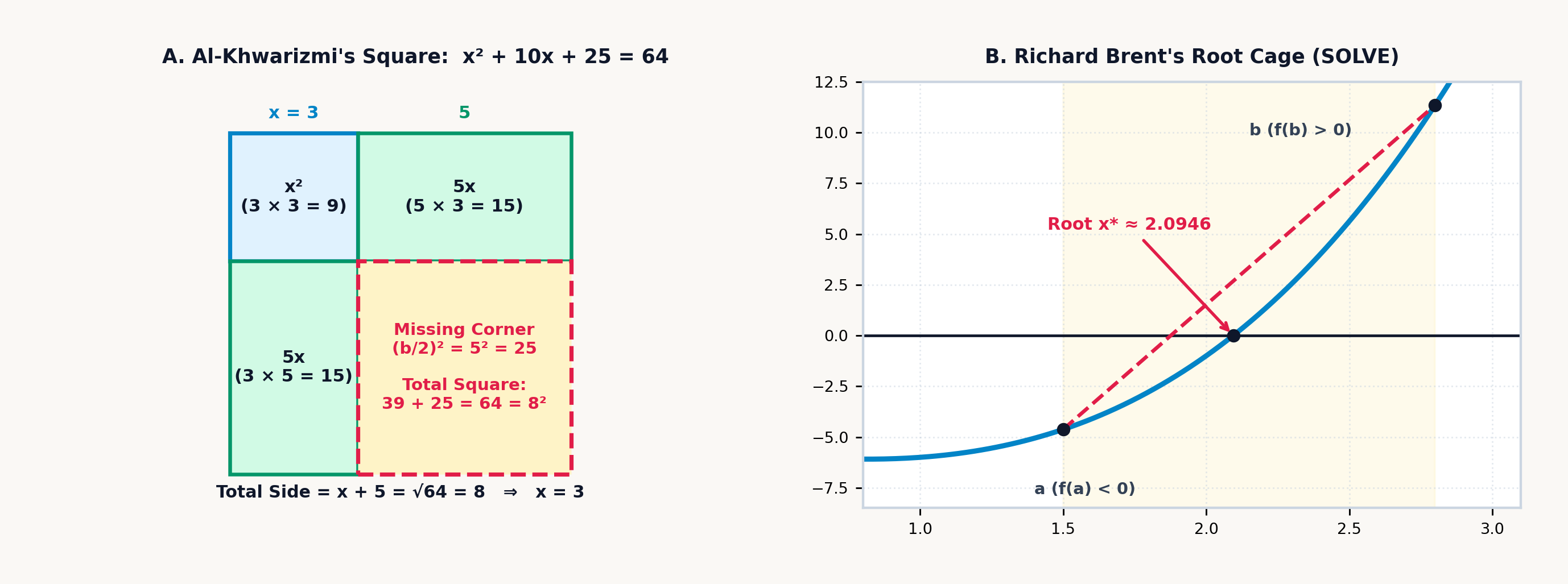
interpreting \(x^2\) as a physical square of side \(x\) and \(10x\) as the area of an attached rectangle folds multiple powers of \(x\) into a single power—the opening step in an algebraic arc that ran from completing the square and Cardano's 1545 Ars Magna (Cardano, 1545) to the fifth-degree radical barrier and Richard Brent's 1973 hybrid root-finding algorithm (Brent, 1973).

7.1 Closed-Form Polynomials, Viète's Identities & Horner's Scheme

To find the positive root \(x\) when \(x^2 + 10x = 39\), split the linear coefficient \(10\) into two equal halves (\(10/2 = 5\)) and add the square of that half-coefficient (\(5^2 = 25\)) to both sides of the equation (Figure 7.1). Adding \(25\) completes the binomial square \((x + 5)^2\) on the left and balances \(39 + 25 = 64\) on the right:

\[(x + 5)^2 = 39 + 25 = 64 = 8^2 \implies x + 5 = \pm 8 \implies \mathbf{x_1 = 3}, \quad \mathbf{x_2 = -13} \tag{Eq. 7.2}\]

When the square is completed on the general quadratic equation \(a x^2 + b x + c = 0\)—or when the equation is divided through by \(a\) to form the reduced monic quadratic \(x^2 + 2px + q = 0\) in terms of the half-linear coefficient \(p = \frac{b}{2a}\) and constant ratio \(q = \frac{c}{a}\)—it yields both the classical quadratic formula and its single-entry half-linear form, where \(p\) and \(q\) each appear only once:

\[x = \frac{-b \pm \sqrt{b^2 - 4ac}}{2a} = -p \pm \sqrt{p^2 - q} \qquad \left(p = \frac{b}{2a},\;\; q = \frac{c}{a}\right) \tag{Eq. 7.3}\]

In factored form, \(a(x - r_1)(x - r_2) = ax^2 - a(r_1 + r_2)x + a r_1 r_2 = 0\) links the roots \((r_1, r_2)\) to the polynomial coefficients through Viète's identities without solving for the individual roots at all:

\[r_1 + r_2 = -\frac{b}{a}, \qquad r_1 r_2 = \frac{c}{a}, \qquad \frac{1}{r_1} + \frac{1}{r_2} = \frac{r_1 + r_2}{r_1 r_2} = -\frac{b}{c}, \qquad r_1^2 + r_2^2 = (r_1 + r_2)^2 - 2r_1 r_2 = \left(\frac{b}{a}\right)^2 - \frac{2c}{a} \tag{Eq. 7.4}\]

Whenever an engineering analysis or mathematics competition asks for a symmetric combination of the roots—such as their sum, product, reciprocal sum, or sum of squares—Viète's identities resolve the answer by inspection: on \(2x^2 - 7x + 4 = 0\), the roots satisfy \(r_1 + r_2 = \mathbf{3.5}\), \(r_1 r_2 = \mathbf{2}\), reciprocal sum \(\frac{1}{r_1} + \frac{1}{r_2} = \frac{7}{4} = \mathbf{1.75}\), and squared sum \(r_1^2 + r_2^2 = 3.5^2 - 2(2) = \mathbf{8.25}\) without extracting any square roots.

7.1.1 Catastrophic Cancellation in the Quadratic Formula

In finite-precision floating-point arithmetic, the classical quadratic formula \(x = \frac{-b \pm \sqrt{b^2 - 4ac}}{2a}\) exhibits a severe numerical instability whenever \(b^2\) is much larger than \(4ac\) (\(b^2 \gg |4ac|\)).

When \(b > 0\) and \(4ac\) is tiny compared to \(b^2\), the radical \(\sqrt{b^2 - 4ac}\) is nearly equal to \(b\). Evaluating the root with the plus sign (\(-b + \sqrt{b^2 - 4ac}\)) subtracts two nearly equal numbers and cancels up to half or more of a floating-point register's significant digits through catastrophic cancellation. Avoiding this loss of significance requires never subtracting \(\sqrt{b^2 - 4ac}\) from a number of the same sign.

Instead, we introduce the sign function \(\operatorname{sgn}(b)\) (which equals \(+1\) when \(b \ge 0\) and \(-1\) when \(b < 0\)) to form the Citardauq ("Quadratic" spelled backward) intermediate quantity \(q\), and then extract the larger-magnitude root \(x_1 = q/a\) and the smaller-magnitude root \(x_2 = c/q\) via Viète's root-product identity \(x_1 x_2 = \frac{c}{a}\):

\[q = -\frac{1}{2}\Big(b + \operatorname{sgn}(b)\sqrt{b^2 - 4ac}\Big), \qquad x_1 = \frac{q}{a}, \qquad x_2 = \frac{c}{q} \tag{Eq. 7.5}\]

Multiplying the radical \(\sqrt{b^2 - 4ac}\) by \(\operatorname{sgn}(b)\) guarantees that \(\operatorname{sgn}(b)\sqrt{b^2 - 4ac}\) always carries the exact same algebraic sign as \(b\), so the two terms inside the parentheses always add in magnitude instead of canceling. Because \(q\) is formed by pure magnitude addition, both \(x_1 = q/a\) and \(x_2 = c/q\) retain every guard digit of precision even when \(b^2\) exceeds \(4ac\) by ten orders of magnitude. On the benchmark \(x^2 + 10x - 39 = 0\) (\(a = 1, b = 10, c = -39\)), the discriminant \(\Delta = b^2 - 4ac = 256\) has square root \(16\), so \(q = -\frac{1}{2}(10 + 16) = \mathbf{-13}\) (\(x_1 = q/a\)) and \(x_2 = c/q = -39 / (-13) = \mathbf{3}\).

Quadratic equations govern two inverse problems in mechanics and forensic engineering: inverse ballistic trajectories and highway stopping distance reconstruction. Forward ballistics projects where a shell lands when its launch angle \(\theta\) is already known; the inverse ballistic problem fixes the target coordinates \((x, y)\) on an elevated ridge at horizontal range \(x\) and vertical elevation \(y\), given a known muzzle speed \(v_0\) and downward gravitational acceleration \(g \approx 9.81\text{ m/s}^2\), and solves backward for the required launch angle \(\theta\). Were the shell fired horizontally in vacuum without gravity, it would climb along the straight line-of-sight tangent \(x\tan\theta\); over flight time \(t = \frac{x}{v_0\cos\theta}\), however, gravity pulls the shell downward by \(\frac{1}{2}gt^2 = \left(\frac{gx^2}{2v_0^2}\right)\sec^2\theta\), where the baseline vertical drop \(d_g = \frac{gx^2}{2v_0^2}\) is the distance the projectile would fall if fired horizontally at speed \(v_0\). Substituting the trigonometric identity \(\sec^2\theta = 1 + \tan^2\theta\) into the parabolic trajectory \(y = x\tan\theta - \frac{gx^2}{2v_0^2}\sec^2\theta\) converts the unknown launch slope \(u = \tan\theta\) into a quadratic equation:

\[\left(\frac{gx^2}{2v_0^2}\right) u^2 - x u + \left(y + \frac{gx^2}{2v_0^2}\right) = 0 \tag{Eq. 7.6}\]

Tilting the barrel steeper increases the flight time across range \(x\) and amplifies gravitational drop through the quadratic term \(\frac{gx^2}{2v_0^2} u^2\), while the linear term \(-xu\) tracks the straight line-of-sight climb and the constant term \(\left(y + \frac{gx^2}{2v_0^2}\right)\) combines the ridge elevation \(y\) with the baseline gravity drop \(d_g\). Whenever the target lies within range, the two positive roots give the gunner two distinct paths to the same coordinates: a flat, fast direct-fire trajectory (\(\theta_1 = \arctan u_1\)) and a high, plunging mortar arc (\(\theta_2 = \arctan u_2\)) that descends from above.

A similar quadratic governs highway braking and reaction stopping distance. When a driver spots a hazard on the highway, the vehicle of mass \(m\) travels at its initial speed \(v_0\) during the human perception-reaction time \(t_r\), covering a linear reaction distance \(d_{\text{react}} = v_0 t_r\). Once the brakes lock, tire-pavement friction (with coefficient \(\mu\) and normal weight \(mg\)) exerts a constant retarding force \(\mu mg\); to bring the vehicle to a halt, the linear friction work \(\mu m g\,d_{\text{brake}}\) must absorb the entire translational kinetic energy \(\frac{1}{2}mv_0^2\), which makes the braking distance \(d_{\text{brake}} = \frac{v_0^2}{2\mu g}\) scale with the square of initial speed \(v_0\) while vehicle mass \(m\) cancels out. Summing reaction and braking distances gives the total stopping distance \(d = v_0 t_r + \frac{v_0^2}{2\mu g}\). When crash investigators measure the total stopping distance \(d\) at the scene, reconstructing the vehicle's unknown initial speed \(v_0\) requires clearing the denominator \(2\mu g\) to extract the positive root of the monic quadratic:

\[v_0^2 + (2\mu g t_r)\, v_0 - 2\mu g d = 0 \tag{Eq. 7.7}\]

Clearing the denominator \(2\mu g\) pits the quadratic kinetic-energy braking term \(v_0^2\) and the linear human-reaction term \((2\mu g t_r)v_0\) against the scaled stopping distance \(2\mu g d\), isolating the pre-braking speed as the unique positive root \(v_0 = -\mu g t_r + \sqrt{(\mu g t_r)^2 + 2\mu g d}\).

7.1.2 The 1535 Milanese Cubic Contest, Cardano's Formula & Casus Irreducibilis

Fior had set all thirty of his 1535 challenge problems as variations of del Ferro's single depressed form \(t^3 + pt = q\); Tartaglia had posed several different families of cubics, including \(t^3 + pt^2 = q\). Expanding the binomial cube \((u - v)^3\) and regrouping its terms yields the algebraic identity:

\[(u - v)^3 + 3uv(u - v) = u^3 - v^3 \tag{Eq. 7.8}\]

Tartaglia saw that setting \(t = u - v\), \(3uv = p\), and \(u^3 - v^3 = -q\) reduces the depressed cubic \(t^3 + pt + q = 0\) to a quadratic equation in \(u^3\).

News of Tartaglia's victory reached the Milanese physician and algebraist Gerolamo Cardano, who persuaded Tartaglia in 1539 to share his rule (encoded in a twenty-five-line poem). Cardano then combined Tartaglia's rule with his own discovery that any full cubic \(A x^3 + B x^2 + C x + D = 0\) can be stripped of its quadratic \(x^2\) term by translating the coordinate origin to the curve's point of inflection via \(x = t - \frac{B}{3A}\). Geometrically, every cubic curve is an S-shaped wave that bends concave-down on one side and concave-up on the other, switching concavity at a unique central balance point where the second derivative \(6Ax + 2B\) vanishes (\(x = -\frac{B}{3A}\)). Sliding the horizontal coordinate axis to that inflection point centers the S-curve symmetrically so the quadratic \(t^2\) term cancels out, leaving only the depressed slope parameter \(p\) and vertical inflection offset \(q\):

\[t^3 + p t + q = 0, \qquad p = \frac{3AC - B^2}{3A^2}, \qquad q = \frac{27A^2D - 9ABC + 2B^3}{27A^3} \tag{Eq. 7.9}\]

Centering the cubic at \(t = 0\) gives \(p\) and \(q\) a direct geometric meaning: the linear coefficient \(p\) is the exact slope of the cubic right at its inflection center (which must be negative, \(p < 0\), for the S-curve to turn backward and form a local hill and valley), while the constant term \(q\) is the vertical height of that inflection point above or below the horizontal axis. Cardano and his pupil Lodovico Ferrari, who soon discovered how to solve the fourth-degree quartic equation by reducing it to a resolvent cubic, now possessed the complete analytical solution to every polynomial up to degree four. After inspecting Scipione del Ferro's posthumous papers in Bologna and verifying that del Ferro had discovered the depressed cubic formula twenty years before Tartaglia, Cardano published the complete cubic and quartic solutions in his 1545 treatise Ars Magna (Cardano, 1545), crediting both del Ferro and Tartaglia.

Solving Tartaglia's simultaneous conditions \(u^3 - v^3 = -q\) and \(u^3(-v^3) = -(p/3)^3\) via the quadratic formula yields \(u^3 = -\frac{q}{2} + \sqrt{\Delta}\) and \(-v^3 = -\frac{q}{2} - \sqrt{\Delta}\), governed by the cubic discriminant \(\Delta = \left(\frac{q}{2}\right)^2 + \left(\frac{p}{3}\right)^3\). Taking the cube roots to recover \(t = u - v\) produces Cardano's cubic formula, inside which appeared an algebraic paradox that forced the recognition of complex numbers:

\[t = \sqrt[3]{-\frac{q}{2} + \sqrt{\Delta}} + \sqrt[3]{-\frac{q}{2} - \sqrt{\Delta}}, \qquad \Delta = \left(\frac{q}{2}\right)^2 + \left(\frac{p}{3}\right)^3 \tag{Eq. 7.10}\]

The two cube-root radicals in Cardano's formula are Tartaglia's \(u\) and \(-v\), while the cubic discriminant \(\Delta\) pits the squared half-offset \((q/2)^2\) against the cubed third-slope \((p/3)^3\) to govern the nature of the three roots across three distinct regimes. When \(\Delta > 0\), the vertical offset \(q\) shifts the inflection center far enough above or below the axis that the S-shaped cubic crosses the horizontal axis only once, yielding one real root and two complex conjugate roots formed by rotating \(u = \sqrt[3]{-q/2 + \sqrt{\Delta}}\) and \(-v = \sqrt[3]{-q/2 - \sqrt{\Delta}}\) by the cube roots of unity \(\omega = -\frac{1}{2} + i\frac{\sqrt{3}}{2}\) and \(\omega^2\). When \(\Delta = 0\), the hilltop or valley floor grazes the horizontal axis tangentially and produces three real roots with at least one repeated root, as in the critically damped RLC filter polynomial \(s^3 + 12s^2 + 45s + 50 = (s+2)(s+5)^2 = 0\) with a repeated double root at \(s = -5\).

When \(\Delta < 0\), the regime known as casus irreducibilis, \(p\) is negative enough that \((p/3)^3\) outweighs \((q/2)^2\), so the S-curve's hill and valley straddle the horizontal axis and cross it three times to produce three distinct real roots (as in \((x-1)(x-2)(x-3) = x^3 - 6x^2 + 11x - 6 = 0\)), yet the discriminant \(\Delta\) under the square root is negative. Extracting those three real numbers from Cardano's formula requires passing through the complex plane and taking the cube root of a complex number \(r e^{i\theta}\) by De Moivre's angle trisection \(r^{1/3}[\cos(\theta/3) + i\sin(\theta/3)]\), where the imaginary parts of the two conjugate cube roots cancel to zero.

7.1.3 Viète's Trigonometric Trisection & Ferrari's Quartic

The complex radicals of casus irreducibilis can be bypassed through trigonometry, because the depressed cubic \(t^3 + pt + q = 0\) (when \(\Delta < 0\), so \(p < 0\)) shares the algebraic structure of the trigonometric triple-angle identity for cosine:

\[\cos(3\theta) = 4\cos^3\theta - 3\cos\theta \implies \cos^3\theta - \frac{3}{4}\cos\theta - \frac{1}{4}\cos(3\theta) = 0 \tag{Eq. 7.11}\]

Scaling the unknown as \(t = 2\sqrt{-p/3}\,\cos\theta\) (Viète's trigonometric solution) matches the depressed cubic to the triple-angle cosine identity term-for-term and expresses all three real roots \(t_0, t_1, t_2\) in closed form without complex square roots:

\[t_k = 2\sqrt{-\frac{p}{3}} \cos\left(\frac{1}{3}\arccos\left(\frac{3q}{2p}\sqrt{-\frac{3}{p}}\right) - \frac{2\pi k}{3}\right), \qquad k = 0, 1, 2 \tag{Eq. 7.12}\]

Geometrically, the outer amplitude factor \(2\sqrt{-p/3}\) sets the horizontal width of the cubic's S-bend between its local extrema; the inner inverse cosine \(\arccos\!\left(\frac{3q}{2p}\sqrt{-3/p}\right)\) measures the phase angle set by the vertical offset \(q\) relative to the hilltop height; and dividing that angle by \(3\) while stepping \(k = 0, 1, 2\) by \(\frac{2\pi k}{3}\) (\(120^\circ\)) trisects the angle on the unit circle and projects the three \(120^\circ\)-spaced vertices of an inscribed equilateral triangle onto the horizontal real axis.

For a fourth-degree quartic equation (such as \(x^4 + 6x^2 + 36 = 60x\)), Lodovico Ferrari discovered how to factor the quartic into two quadratics by introducing an adjustable auxiliary parameter \(y\) that turns the equation into a difference of two squares. First, shifting the horizontal coordinate removes the cubic \(x^3\) term to leave the depressed quartic \(x^4 + px^2 + qx + r = 0\) with quadratic coefficient \(p\), linear tilt \(q\), and constant term \(r\). Moving \(px^2 + qx + r\) to the right side, completing the square on the left as \((x^2 + \frac{p}{2})^2\), and inserting an auxiliary variable \(y\) inside the left-hand square yields:

\[\left(x^2 + \frac{p}{2} + y\right)^2 = (p + 2y)x^2 - qx + \left(\frac{p^2}{4} - r + py + y^2\right) \tag{Eq. 7.13}\]

The left-hand side is already a perfect square for every choice of \(y\), while the right-hand side is an ordinary quadratic in \(x\) with \(x^2\)-coefficient \(A = (p + 2y)\), \(x\)-coefficient \(B = -q\), and constant term \(C = \left(\frac{p^2}{4} - r + py + y^2\right)\). We are free to choose \(y\) so that this right-hand quadratic also becomes a perfect square \((mx + n)^2\)—which happens whenever its quadratic discriminant \(B^2 - 4AC\) equals zero:

\[q^2 - 4(p + 2y)\left(y^2 + py + \frac{p^2}{4} - r\right) = 0 \tag{Eq. 7.14}\]

Multiplying out \((p + 2y)\) by the quadratic in \(y\) makes this condition a third-degree cubic equation in \(y\)—the resolvent cubic—which Cardano's cubic formula solves in closed form. Once one root \(y_1\) of the resolvent cubic is found, the right-hand side locks into \((mx + n)^2\), turning the quartic into the difference of two squares \((x^2 + \frac{p}{2} + y_1)^2 - (mx + n)^2 = 0\), which splits into the two quadratic equations \(x^2 + \frac{p}{2} + y_1 = \pm(mx + n)\) to yield all four roots.

For any cubic (\(A x^3 + B x^2 + C x + D = 0\)) with roots \(r_1, r_2, r_3\), Viète's root-coefficient formulas verify the roots without substituting each value back into the polynomial. Expanding \(A(x - r_1)(x - r_2)(x - r_3) = A x^3 - A(r_1 + r_2 + r_3)x^2 + A(r_1 r_2 + r_2 r_3 + r_3 r_1)x - A r_1 r_2 r_3\) and matching coefficients term by term yields the sum of roots (trace), pairwise product sum, and product of roots (determinant):

\[r_1 + r_2 + r_3 = -\frac{B}{A}, \qquad r_1 r_2 + r_2 r_3 + r_3 r_1 = +\frac{C}{A}, \qquad r_1 \cdot r_2 \cdot r_3 = -\frac{D}{A} \tag{Eq. 7.15}\]

On our benchmark cubic \(x^3 - 6x^2 + 11x - 6 = 0\) with roots \(1, 2, 3\), summing the three real parts gives the trace \(1 + 2 + 3 = 6 = -(-6)/1\), their pairwise product sum is \(1(2) + 2(3) + 3(1) = 11 = +11/1\), and their determinant product is \(1 \times 2 \times 3 = 6 = -(-6)/1\). In any depressed cubic \(t^3 + pt + q = 0\) (where \(B = 0\)), the three roots always sum to zero (\(t_1 + t_2 + t_3 = 0\)), because the coordinate shift \(x = t - \frac{B}{3A}\) places the origin at the centroid of the three roots.

That chain of radical reductions stops permanently after the degree-4 quartic, and no general radical formula exists for a degree-5 quintic equation (\(Ax^5 + Bx^4 + Cx^3 + Dx^2 + Ex + F = 0\)). For a degree-2 quadratic, the resolvent has degree 1; for a degree-3 cubic, Tartaglia's resolvent has degree 2; for a degree-4 quartic, Ferrari's resolvent has degree 3. In each case, the auxiliary equation has lower degree than the original polynomial. When the same permutation method is applied to a degree-5 quintic, however, the resolvent equation jumps up to degree 6 (with \(5!/2 = 60\) alternating permutations).

By the Abel–Ruffini and Galois theorem, this barrier is structural and absolute. For degrees \(n = 2, 3, 4\), the permutation group \(S_n\) of the roots decomposes into commutative cyclic quotients ("solvable groups") that correspond to extracting \(k\)-th roots \(\sqrt[k]{\phantom{x}}\). For \(n \ge 5\), however, the alternating group \(A_5\), which is isomorphic to the \(60\) rotational symmetries of a regular icosahedron, is a simple non-abelian group that cannot be factored into cyclic steps. No general radical formula in \(+, -, \times, \div\), and \(\sqrt[n]{\phantom{x}}\) can exist for degree 5 or higher.

7.1.4 Evaluating Polynomials from the Inside Out: Horner's Nested Scheme

Before solving a polynomial equation \(P(x) = 0\), one needs an efficient, numerically stable method to evaluate \(P(x)\) at any argument \(x = x_0\), illustrated by the general fourth-degree quartic polynomial:

\[P(x) = a_4 x^4 + a_3 x^3 + a_2 x^2 + a_1 x + a_0 \tag{Eq. 7.16}\]

When \(P(x)\) is evaluated term by term as written (\(x^4\) multiplied by \(a_4\), plus \(x^3\) multiplied by \(a_3\), plus \(x^2\) multiplied by \(a_2\), and so on), it repeats power computations unnecessarily (\(4 + 3 + 2 + 1 = 10\) multiplications, or three separate exponentiations). Worse, near a root where large positive and negative power terms nearly cancel, computing \(a_n x^n\) separately magnifies floating-point rounding error.

Recursive factoring of \(x\) from the inside out transforms the polynomial into Horner's nested scheme:

\[P(x) = a_4 x^4 + a_3 x^3 + a_2 x^2 + a_1 x + a_0 = \Big(\big((a_4 x + a_3)x + a_2\big)x + a_1\Big)x + a_0 \tag{Eq. 7.17}\]

In Horner's nested scheme, every explicit exponent vanishes. To evaluate any degree-\(n\) polynomial at \(x_0\), you start with the leading coefficient \(b_n = a_n\) and repeat a two-step linear recurrence \(b_k = b_{k+1} x_0 + a_k\) exactly \(n\) times, multiplying the running value by \(x_0\) and adding the next coefficient \(a_k\).

Across the four nested stages of a quartic \(P(x_0) = (((a_4 x_0 + a_3)x_0 + a_2)x_0 + a_1)x_0 + a_0\), the running accumulator starts with \(b_4 = a_4\), multiplies by \(x_0\), and adds \(a_3\) in the first stage to form \(b_3 = a_4 x_0 + a_3\); multiplies \(b_3\) by \(x_0\) and adds \(a_2\) in the second stage to form \(b_2 = b_3 x_0 + a_2\); multiplies \(b_2\) by \(x_0\) and adds \(a_1\) in the third stage to form \(b_1 = b_2 x_0 + a_1\); and finally multiplies \(b_1\) by \(x_0\) and adds \(a_0\) to reach the remainder \(b_0 = b_1 x_0 + a_0 = P(x_0)\). This recurrence requires four multiplications, four additions, zero powers, and zero temporary variables.

Each intermediate value \((b_4, b_3, b_2, b_1)\) produced at each step of Horner's recurrence has direct algebraic meaning: they are the exact coefficients of the cubic quotient polynomial \(Q(x)\) obtained by Horner synthetic division when dividing \(P(x)\) by \((x - x_0)\):

\[P(x) = (x - x_0)\,Q(x) + b_0 = (x - x_0)\left(b_4 x^3 + b_3 x^2 + b_2 x + b_1\right) + P(x_0) \tag{Eq. 7.18}\]

This Polynomial Remainder Theorem identity \(P(x) = (x - x_0)Q(x) + P(x_0)\) provides polynomial deflation, simultaneous derivative evaluation, and suppression of catastrophic cancellation near multiple roots. Once one exact root \(r_1\) of a polynomial is found (where the remainder \(P(r_1) = 0\)), the intermediate numbers generated during Horner's evaluation at \(r_1\) supply the deflated degree-\((n-1)\) quotient polynomial \(Q(x) = P(x)/(x - r_1)\), which reduces a fourth-degree quartic to a cubic or a cubic to a quadratic. Differentiating \(P(x) = (x - x_0)Q(x) + P(x_0)\) with respect to \(x\) by the product rule yields:

\[P'(x) = Q(x) + (x - x_0)Q'(x) \implies P'(x_0) = Q(x_0) \tag{Eq. 7.19}\]

A second Horner pass on the intermediate coefficients evaluates the quotient polynomial \(Q(x)\) at \(x_0\) and therefore gives the exact derivative \(P'(x_0)\) without a separate symbolic derivative formula. In computational thermodynamics and flight-control engineering—where computers evaluate standard-atmosphere pressure-altitude curves \(P(h) = a_3 h^3 + a_2 h^2 + a_1 h + a_0\) and NASA Glenn molar heat-capacity fits \(C_p(T)/R = a_0 + a_1 T + a_2 T^2 + a_3 T^3 + a_4 T^4\)—nested Horner evaluation also suppresses cancellation near repeated roots (such as \(s = -5\) in the critically damped RLC filter) by updating the local factor \((s + 5)\) at each step without subtracting large, independently rounded powers \(s^3\) and \(12s^2\).

Nested factoring also simplifies rational formulas and symmetric high-degree equations across physics. In a silicon photovoltaic cell, the Fill Factor \(FF\) measures how "square" the current-voltage curve is—defined as the ratio of maximum usable electrical power \(P_{\max}\) to the theoretical rectangle product of open-circuit voltage \(V_{\text{oc}}\) and short-circuit current \(I_{\text{sc}}\). Although the maximum power point satisfies a transcendental diode equation that cannot be inverted in closed form, dividing \(V_{\text{oc}}\) by the junction's thermal voltage \(V_T = k_B T / q\) (\(\approx 25.85\text{ mV}\) at \(300\text{ K}\)) defines the dimensionless normalized open-circuit voltage \(v_{\text{oc}} = V_{\text{oc}} / V_T\) and yields Martin Green's accurate rational-logarithmic expression for \(FF\):

\[\text{Fill Factor } FF = \frac{v_{\text{oc}} - \ln(v_{\text{oc}} + 0.72)}{v_{\text{oc}} + 1} \tag{Eq. 7.20}\]

As the normalized open-circuit voltage \(v_{\text{oc}}\) grows large compared to the thermal scale \(V_T\), the leading fraction \(\frac{v_{\text{oc}}}{v_{\text{oc}} + 1}\) approaches an ideal square curve (\(FF \to 1\)), while subtracting \(\ln(v_{\text{oc}} + 0.72)\) before dividing by \(v_{\text{oc}} + 1\) accounts for the voltage rounded off at the exponential diode knee near maximum power. Likewise, when two coupled undamped spring-mass pendulums with stiffness matrix \(\mathbf{K}\) and mass matrix \(\mathbf{M}\) vibrate harmonically at natural angular frequency \(\omega\), the characteristic eigenvalue equation \(\det(\mathbf{K} - \omega^2\mathbf{M}) = 0\) expands into a biquadratic polynomial containing only even powers of frequency (\(a \omega^4 + b \omega^2 + c = 0\)), which reduces immediately to a quadratic in the squared frequency \(u = \omega^2\) whose positive square roots \(\omega = \sqrt{u}\) give the two normal-mode vibration frequencies.

---

7.2 Iterative Root-Finding & Implicit Physical Laws

Once a polynomial reaches degree five (such as \(x^5 - x - 1 = 0\)) or a physical conservation law combines algebraic powers \(x\) with sines, cosines, exponentials, and logarithms in a transcendental equation, no symbolic manipulation can isolate the unknown on one side of the equals sign.

When symbolic algebra cannot invert \(f(x)\) to solve \(f(x^*) = 0\), numerical root-finding relies on two contrasting strategies: interval bisection and local tangent or secant extrapolation. When a continuous curve \(f(x)\) lies below the axis at \(x = a\) with \(f(a) < 0\) and above it at \(x = b\) with \(f(b) > 0\), so that \(f(a)\cdot f(b) < 0\), the Intermediate Value Theorem guarantees that the curve crosses \(y = 0\) at least once inside the bracket \([a, b]\).

The Bisection Method evaluates the function at the midpoint \(m = \frac{1}{2}(a + b)\), inspects its sign, and discards whichever half does not contain the sign change. Every step halves the uncertainty and gains \(1\text{ binary bit}\) of precision per step (linear convergence, order \(p = 1\)). After \(40\) bisections, the bracket shrinks by \(2^{-40} \approx 10^{-12}\), though requiring \(40\) to \(50\) evaluations makes bisection slow.

To accelerate convergence on smooth curves (such as the cubic benchmark \(x^3 - 2x - 5 = 0\) near \(x_0 = 2\)), the Newton–Raphson method evaluates both the residual height \(f(x_n)\) of the curve above or below the horizontal axis at the current guess \(x_n\) and the local tangent slope \(f'(x_n)\), stepping along that tangent line to where it crosses \(y = 0\) at \(x_{n+1}\):

\[x_{n+1} = x_n - \frac{f(x_n)}{f'(x_n)} \tag{Eq. 7.21}\]

Dividing the vertical residual height \(f(x_n)\) by the local tangent slope \(f'(x_n)\) (rise over run) recovers the horizontal run \(\Delta x = f(x_n)/f'(x_n)\) needed to slide down the tangent line to its \(x\)-axis intercept \(x_{n+1}\). Near a simple root, the Newton-Raphson method is quadratically convergent (\(p = 2\)) and doubles the number of accurate decimal digits on every step (\(1 \to 2 \to 4 \to 8 \to 16\text{ digits}\)). When the analytic derivative \(f'(x)\) is unavailable, replacing the tangent slope with the Secant Chord through the last two iterates yields superlinear convergence at the golden-ratio exponent \(p = \phi = \frac{1+\sqrt{5}}{2} \approx 1.618\).

The vulnerability of Newton-Raphson and the Secant Method lies in the slope denominator \(f'(x_n)\) (or \(f(x_n) - f(x_{n-1})\)). Whenever an iterate lands near a local extremum, an inflection plateau, or a horizontal asymptote where the slope flattens out (\(f'(x_n) \approx 0\)), the nearly horizontal tangent line projects the next estimate \(x_{n+1}\) far outside the region of interest or into an oscillatory cycle.

When an equation can be rearranged into the self-referential form \(x = g(x)\), the Contraction Mapping Theorem guarantees that repeatedly feeding the output back into the function (\(x_{n+1} = g(x_n)\)) spirals or staircases into a unique fixed point \(x^* = g(x^*)\) whenever the local slope satisfies \(|g'(x^*)| < 1\). In radian mode, iterating \(x_{n+1} = \cos(x_n)\) from any starting value traces a converging cobweb spiral (1, 0.54, 0.858, 0.654, \(\dots\)) to the universal transcendental Dottie number \(x^* = \cos(x^*) \approx \mathbf{0.739\text{ rad}}\) (where \(|\sin(0.739)| \approx 0.674 < 1\)), while a self-similar infinite nested radical \(x = \sqrt{c + \sqrt{c + \sqrt{c + \dots}}}\) satisfies the fixed-point relation \(x = \sqrt{c + x} \implies x^2 - x - c = 0\) with positive root \(x = \frac{1 + \sqrt{1 + 4c}}{2}\) (so \(\sqrt{6 + \sqrt{6 + \dots}} = \mathbf{3}\) and \(\sqrt{1 + \sqrt{1 + \dots}} = \varphi \approx \mathbf{1.618}\)). Whenever \(|g'(x^*)| > 1\), however, direct fixed-point iteration repels away from the root, so a bracketed root-finder must be applied to \(f(x) = g(x) - x = 0\).

7.2.1 Richard Brent's 1973 Hybrid Root-Finding Algorithm

In 1973, Richard P. Brent demonstrated in Algorithms for Minimization Without Derivatives (Brent, 1973) how to combine the guaranteed bracketing of Bisection with the superlinear convergence of Interpolation so that the solver achieves rapid convergence on smooth curves, requires no derivatives, and never diverges outside its bracket. This hybrid bracketing philosophy was soon adapted for scientific pocket calculators (Kahan, 1979; HP, 1982; Evett et al., 1983; HP, 1991), pairing derivative-free bracketing with post-convergence residual diagnostics.

Brent's hybrid root-finding algorithm combines inverse quadratic interpolation with five acceptance tests. Given three distinct points \((a, f(a))\), \((b, f(b))\), and \((c, f(c))\) near the root, fitting an ordinary upright parabola \(y = P(x)\) can fail whenever its vertex turns around before reaching the \(x\)-axis and yields no real roots.

To avoid that failure, Brent reverses the roles of the axes and fits \(x\) sideways as a Lagrange quadratic polynomial of \(y\) (\(x = P(y)\)) passing through the three inverted pairs \((f(a), a)\), \((f(b), b)\), and \((f(c), c)\), then evaluates that sideways parabola right at the horizontal axis \(y = 0\) to obtain the next root estimate \(x_{\text{IQI}}\):

\[x_{\text{IQI}} = \frac{a f(b) f(c)}{(f(a)-f(b))(f(a)-f(c))} + \frac{b f(a) f(c)}{(f(b)-f(a))(f(b)-f(c))} + \frac{c f(a) f(b)}{(f(c)-f(a))(f(c)-f(b))} \tag{Eq. 7.22}\]

Each bracket coordinate \(a, b,\) or \(c\) is weighted by the product of the residuals at the other two points divided by the pairwise residual differences. As the best estimate \(b\) closes in on the true root so that \(f(b) \to 0\), the factor \(f(b)\) in the first and third terms drives the weights on \(a\) and \(c\) toward zero while the middle weight \(\frac{f(a)f(c)}{(f(b)-f(a))(f(b)-f(c))}\) approaches \(1\), locking \(x_{\text{IQI}}\) onto the root crossing. At \(y = 0\), a sideways parabola always yields a single unique real number \(x_{\text{IQI}}\) and converges at order \(p \approx 1.839\), nearly doubling the number of significant digits per step.

To guard against wild extrapolations, the algorithm keeps the root enclosed inside a contracting sign-change bracket \([a, b]\) where \(f(a)f(b) \le 0\). Whenever Secant or Inverse Quadratic Interpolation proposes a trial step \(s\), five acceptance conditions verify that \(s\) falls inside the interior three-quarter window \(\left(\frac{3a+b}{4}, b\right)\) and that consecutive steps contract the bracket by at least half every two iterations. If an interpolated step attempts to leave the bracket or stalls on a flat plateau, the algorithm rejects the interpolation and executes a bisection step \(m = \frac{1}{2}(a + b)\).

Root-Finding Algorithm	Convergence Order (\(p\))	Derivative \(f'(x)\) Required	Bracket Guarantee	Behavior Near Flat Slopes (\(f'(x) \approx 0\))
Bisection	\(1\)	No	Yes (Guaranteed)	Steady (\(1\text{ bit/step}\)), immune to slope traps
Newton-Raphson	\(2\)	Yes	No	Catastrophic divergence when \(f'(x) \approx 0\)
Secant Chord	\(\approx 1.618\) (\(\phi\))	No	No	Can fling iterates far outside the search region
Brent's Hybrid Method	\(\approx 1.839\)	No	Yes (Guaranteed)	Instant bisection fallback; zero divergence

7.2.2 Multiple-Root Conditioning and Polynomial Deflation Order

When a curve grazes the horizontal axis tangentially without crossing it at a non-zero slope, floating-point root accuracy is bounded by the local curvature of the root, much like a shoreline where a coastal hillside meets sea level (\(y = 0\)) while tiny ocean ripples of height \(\varepsilon_{\text{mach}} \approx 10^{-16}\) lap against the shore. Where a steep cliff plunges straight into the sea at a simple root (\(f'(x^*) \ne 0\)), a vertical ripple of size \(\varepsilon_{\text{mach}}\) shifts the horizontal waterline by at most \(\Delta x \approx \frac{\varepsilon_{\text{mach}}}{|f'(x^*)|}\). Where a flat sandy beach grazes sea level tangentially like a parabolic trough at an \(m\)-fold repeated root \(f(x) \approx c(x - x^*)^m\) with leading curvature coefficient \(c\), however, setting \(|c||\Delta x|^m \approx \varepsilon_{\text{mach}}\) shows that the same vertical ripple washes the waterline across a much wider horizontal uncertainty band \(\Delta x\):

\[\Delta x \approx \left(\frac{\varepsilon_{\text{mach}}}{|c|}\right)^{1/m} \tag{Eq. 7.23}\]

Because the fractional exponent \(1/m\) extracts the \(m\)-th root of the tiny ratio \(\varepsilon_{\text{mach}}/|c|\), higher multiplicity \(m\) dramatically widens the dead zone: for a double tangent root (\(m = 2\), as in \((x - 3)^2 = 0\)), the horizontal uncertainty widens to the square root of machine epsilon (\(\varepsilon_{\text{mach}}^{1/2} \approx 10^{-8}\)), where half the digits of precision are lost to floating-point rounding noise; for a triple root (\(m = 3\)), precision drops to \(\varepsilon_{\text{mach}}^{1/3} \approx 10^{-5}\).

In polynomial deflation, dividing a high-degree polynomial \(P(x)\) to \(Q(x) = P(x)/(x - r_1)\) by removing its largest root \(|r_1|\) first contaminates the lower coefficients of \(Q(x)\) with rounding errors and perturbs the remaining roots. Deflating roots in increasing order of magnitude (\(|r_1| \le |r_2| \le \dots\)) preserves coefficient accuracy, and solving the derivative \(f'(x) = 0\) at an even-multiplicity tangent minimum restores simple-root conditioning.

7.2.3 Bracketing, False Poles & Residual Verification

An automatic root-finder operates as a two-phase bracketing search followed by a post-convergence residual audit. In the first phase, if two initial guesses \(a\) and \(b\) already straddle a sign change (\(f(a)\cdot f(b) \le 0\)), the interval \([a, b]\) locks in as the starting bracket. When given only a single seed \(x_0\), or two guesses on the same side of the axis where \(f(a)\cdot f(b) > 0\), an outward search generates a companion probe (\(\Delta = 0.1|x_0|\) for \(|x_0| < 1\), or \(\Delta = 0.1\) for \(|x_0| \ge 1\)) and advances outward for up to \(50\) steps using clamped secant steps, or expanding by the golden ratio \(\phi \approx 1.618\) whenever the slope is flat. Along the way, the search retracts any probe that steps outside the domain of \(\ln x\) or \(\sqrt{x}\), and it detects even-multiplicity tangent roots like \((x - 2)^2 = 0\) whenever \(|b - a| < 10^{-12}\) and \(|f(b)| < 10^{-7}\).

In the second phase, once a sign change \(f(a)\cdot f(b) \le 0\) is bracketed, the solver applies Brent's guarded Inverse Quadratic Interpolation (IQI) or Secant Chord step, falling back to a Bisection step \(m = \frac{1}{2}(a + b)\) whenever an interpolated step fails the interior-window or contraction checks, and terminating once \(|f(b)| \le 10^{-13}\) or the half-bracket width reaches machine tolerance \(\text{tol} = 2\varepsilon_{\text{mach}}|b| + \frac{1}{2}\cdot 10^{-12}\).

Three mathematical conditions can prevent a real-axis search from bracketing a sign change. First, on positive-definite or negative-definite curves (such as \(f(x) = x^2 + 4 = 0\), whose roots \(\pm 2i\) are imaginary, or \(f(x) = e^x + 1 = 0\)), \(f(x) > 0\) for every real \(x\), so no sign change exists anywhere on the real line. Second, when an initial seed is separated from the root by an asymptote or domain wall (such as \(\ln x\) or \(\sqrt{f}\) in Colebrook's friction law), seeding far from the physical regime can cause outward probes to bounce repeatedly off the \(x \le 0\) boundary unless two explicit bracket guesses \(a\) and \(b\) are chosen inside the valid domain. Third, at an even-multiplicity tangent root (such as \(f(x) = (x - 3)^4 = 0\)), the curve touches \(y = 0\) without crossing (\(f(a)\cdot f(b) \ge 0\) everywhere); if coarse outward probes step over the tangent point, solving the derivative equation \(f'(x) = 0\) (where the tangent extremum becomes a simple odd-multiplicity crossing) restores guaranteed sign-change bracketing.

The function residual \(f(x^*)\) at the converged point \(x^*\) distinguishes a genuine root from a discontinuous pole. If an initial bracket straddles a vertical asymptote (discontinuous pole) where the curve jumps from \(-\infty\) to \(+\infty\) (such as \(f(x) = \tan x\) across \(x = \pi/2\) or \(f(x) = \frac{1}{x - 2}\) across \(x = 2\)), the opposite signs \(f(a)\cdot f(b) < 0\) on either side of the discontinuity cause bisection to contract around the pole \(x = 2\). Checking the residual \(f(x^*)\) at the reported coordinate separates the two cases: at a true root, the residual vanishes (\(|f(x^*)| \le 10^{-12}\)); at a false pole, the residual explodes (\(|f(x^*)| \gg 1\) or undefined division by zero).

In multi-stage engineering workflows, a solved root \(x^*\) is rarely the final number on the page: an orbital mission planner solves Kepler's equation for the eccentric anomaly \(E^*\) in order to substitute \(E^*\) into the focal radius \(r = a(1 - e\cos E^*)\), and a hydraulic engineer solves Colebrook's equation for the friction factor \(f^*\) in order to multiply \(f^*\) by the dynamic velocity head \(\frac{L}{D}\frac{v^2}{2g}\) already waiting on the stack. Traditional single-line root-finders return three diagnostic outputs at once—the root \(x^*\) in \(X\), the previous iterate in \(Y\), and the function residual \(f(x^*)\) in \(Z\)—which overwrites three levels of the stack and destroys any intermediate constants parked in Registers \(Y\) and \(Z\). On the SC-32, the root-finder lifts the stack by one level to place \(x^*\) into Register \(X\) while preserving the starting seed and two prior stack levels above it, and evaluates the stored equation on demand when a residual pole audit \(f(x^*)\) is needed.

7.2.4 Implicit Transcendental Equations in Fluid Friction & Orbital Mechanics

When a physical question runs in reverse to solve for an internal state variable instead of the output on the left-hand side, conservation laws that were explicit in the forward direction turn into coupled polynomial or transcendental equations.

The van der Waals real-gas law exhibits this structural shift when inverted. An ideal gas of molar volume \(V_m\) at absolute temperature \(T\) and universal gas constant \(R\) obeys \(P V_m = RT\), ignoring both the cohesive attraction between nearby molecules (parameterized by the van der Waals constant \(a\), which pulls molecules together and reduces wall pressure by \(\frac{a}{V_m^2}\)) and the finite hard-sphere volume occupied by the molecules themselves (the excluded covolume \(b\), which shrinks the free container space to \(V_m - b\)). When \(V_m\) and \(T\) are already known, the van der Waals equation of state \(\left(P + \frac{a}{V_m^2}\right)(V_m - b) = RT\) yields the pressure \(P = \frac{RT}{V_m - b} - \frac{a}{V_m^2}\) by a direct arithmetic sequence.

In chemical process design, however, a gauge on the pipeline fixes the operating pressure \(P\) and temperature \(T\), and the engineer must solve backward for the unknown molar volume \(V_m\) (or the dimensionless compressibility factor \(Z = \frac{P V_m}{RT}\), which equals \(1\) for an ideal gas). Because intermolecular attraction \(\frac{a}{V_m^2}\) depends on the inverse square of volume while covolume exclusion \((V_m - b)\) is linear in volume, clearing the denominator multiplies \(V_m^2\) by \((V_m - b)\) and turns the inverse problem into the Cubic Virial Equation of State (with dimensionless attraction \(A = \frac{a P}{(RT)^2}\) and dimensionless covolume \(B = \frac{b P}{RT}\)):

\[Z^3 - (1 + B)Z^2 + A Z - A B = 0 \qquad \Longleftrightarrow \qquad P V_m^3 - (P b + R T)V_m^2 + a V_m - a b = 0 \tag{Eq. 7.24}\]

Multiplying the cohesive pressure \(\frac{a}{V_m^2}\) across \((V_m - b)V_m^2\) introduces the linear \(+a V_m\) and constant \(-ab\) terms alongside the ideal-gas and covolume compression terms \(P V_m^3 - (Pb + RT)V_m^2\). Above the critical temperature, this cubic has one real gas root (\(\Delta > 0\)); below the critical temperature inside the two-phase vapor-liquid dome (\(\Delta < 0\)), it exhibits three distinct real roots where the smallest root represents the dense liquid phase, the middle root is the mechanically unstable spinodal inflection (an unphysical S-bend slope where pressure would rise as volume expands, causing the fluid to separate spontaneously into droplets and vapor), and the largest root represents the saturated vapor phase, so Cardano and Viète's analytical cubic solution is needed to extract all three phases together.

An analogous forward-versus-inverse asymmetry governs elliptical orbital mechanics. When a spacecraft's angular position (true anomaly \(\nu\)) along its elliptical orbit is known, evaluating the focal conic radius \(r(\nu) = \frac{a(1 - e^2)}{1 + e\cos\nu}\) is an explicit trigonometric calculation. Reversing the problem poses the fundamental timing relationship of astrodynamics: given the clock time \(t\) elapsed since perihelion passage (which fixes the uniform mean anomaly \(M = \frac{2\pi t}{T}\) across orbital period \(T\)), determining where the body lies along its elliptical orbit. Projecting the ellipse of eccentricity \(e\) onto its circumscribing auxiliary circle of radius \(a\) defines the geometric eccentric anomaly \(E\), and equating the swept focal sector area to the elapsed fraction of the orbital period yields Kepler's Transcendental Anomaly Equation:

\[M - E + e\sin E = 0 \qquad \Longleftrightarrow \qquad E - e\sin E = M \tag{Eq. 7.25}\]

The eccentric anomaly \(E\) appears simultaneously as a linear algebraic arc (\(E\), from the auxiliary circular sector area \(\frac{1}{2}a^2 E\)) and inside a trigonometric sine (\(e\sin E\), from the focal offset triangle \(\frac{1}{2}a(ae)\sin E\) subtracted when the central body sits at the focus instead of the geometric center). Because no sequence of algebraic operations or inverse trigonometric functions can combine a linear arc and its sine to isolate \(E\), inverting time into orbital position requires an iterative root-finder.

A third fundamental feedback trap governs fluid friction in pipelines of length \(L\), internal diameter \(D\), and gravitational acceleration \(g\), where friction along the wall causes a pressure head loss \(h_f = f\frac{L}{D}\frac{v^2}{2g}\) proportional to the dimensionless Darcy–Weisbach friction factor \(f\). The flow regime is governed by the dimensionless Reynolds number \(\text{Re} = \frac{\rho v D}{\mu}\)—the ratio of fluid inertial momentum (fluid density \(\rho\) times mean flow speed \(v\) times pipe diameter \(D\)) to viscous shear damping (dynamic viscosity \(\mu\)). When a viscous liquid flows slowly in the smooth laminar regime (\(\text{Re} < 2,300\)), parabolic viscous shear integrates to an explicit law where the friction factor is \(f = 64/\text{Re}\). Once a municipal water main, petroleum pipeline, or rocket propellant feedline enters the high-speed turbulent regime (\(\text{Re} > 4,000\)), however, chaotic eddies scrub against the microscopic roughness peaks \(\varepsilon\) of the pipe wall, cushioned only by a thin viscous sublayer whose thickness \(\delta_v \propto \frac{D}{\text{Re}\sqrt{f}}\) shrinks as wall shear stress (and thus \(\sqrt{f}\) itself) grows. Combining smooth-wall turbulent boundary-layer scaling with rough-pipe resistance yields the implicit Colebrook–White Equation (Colebrook, 1939) for the Darcy–Weisbach friction factor \(f\):

\[\frac{1}{\sqrt{f}} = -2 \log_{10} \left( \frac{\varepsilon / D}{3.7} + \frac{2.51}{\text{Re}\sqrt{f}} \right) \tag{Eq. 7.26}\]

Two competing drag mechanisms add together inside the logarithm: the rough-wall turbulent limit \(\frac{\varepsilon/D}{3.7}\), governed by the relative wall roughness height \(\varepsilon/D\) protruding into the core flow at high Reynolds numbers, and the smooth-wall viscous sublayer limit \(\frac{2.51}{\text{Re}\sqrt{f}}\), governed by viscous shear across the thin laminar cushion at the wall. Because the friction factor \(f\) feeds back into the sublayer thickness inside the logarithm, \(\sqrt{f}\) is trapped on both sides of the equation, requiring bracketed root-finding to isolate the turbulent friction factor in municipal pipeline and hydraulic network design.

---

7.3 Hunting Roots on the Four-Register Stack

On the SC-32, closed-form polynomial equations of degree two or three (POLY) are separated from higher-degree and transcendental conservation laws (EQN and SOLVE) so neither requires manual iteration loops.

When the governing relation is a cubic (\(Ax^3 + Bx^2 + Cx + D = 0\)) or quadratic (\(Bx^2 + Cx + D = 0\)) with numerical coefficients, the dedicated Polynomial Solver (POLY) activates a five-button softkey bar to accept coefficients without STO or RCL, and executes the polynomial when you press [XEQ]:

1. Opening the Polynomial Workspace & Softkey Bar: Pressing [↱] [POLY] (the right-shifted function on the [XEQ] key) displays the template Ax^3 + Bx^2 + Cx + D across the top of the LCD and presents the five softkeys: $\(\mathtt{[A]} \quad \mathtt{[B]} \quad \mathtt{[C]} \quad \mathtt{[D]} \quad \mathtt{[CLR]}\)$
2. Default of Zero & Clearing Previous Coefficients (CLR): Every unassigned coefficient slot (A, B, C, D) defaults to 0. If variables A through D already hold values from an earlier calculation, they pre-populate the workspace on entry; tapping the fifth softkey (CLR) clears all four coefficient slots (POLY CLR), removes their assignment markers, and resets every slot back to its default of 0.
3. Entering Coefficients via Softkeys (A•, B•, C•, D•): Type a coefficient's numerical value into Register \(X\) (tapping [+/-] for a negative coefficient) and tap the corresponding softkey (A for \(x^3\), B for \(x^2\), C for \(x\), or D for the constant term) directly, with no need for [STO] or [RCL]. The softkey label gains a bullet dot (A•, B•, C•, D•) to mark which terms have been set. Because unassigned slots default to 0, you never need to enter 0 for missing powers—and to solve a quadratic equation (\(Bx^2 + Cx + D = 0\)), you leave A unassigned at its 0 default, enter the \(x^2\), \(x\), and constant coefficients into softkeys B, C, and D, and press [XEQ].
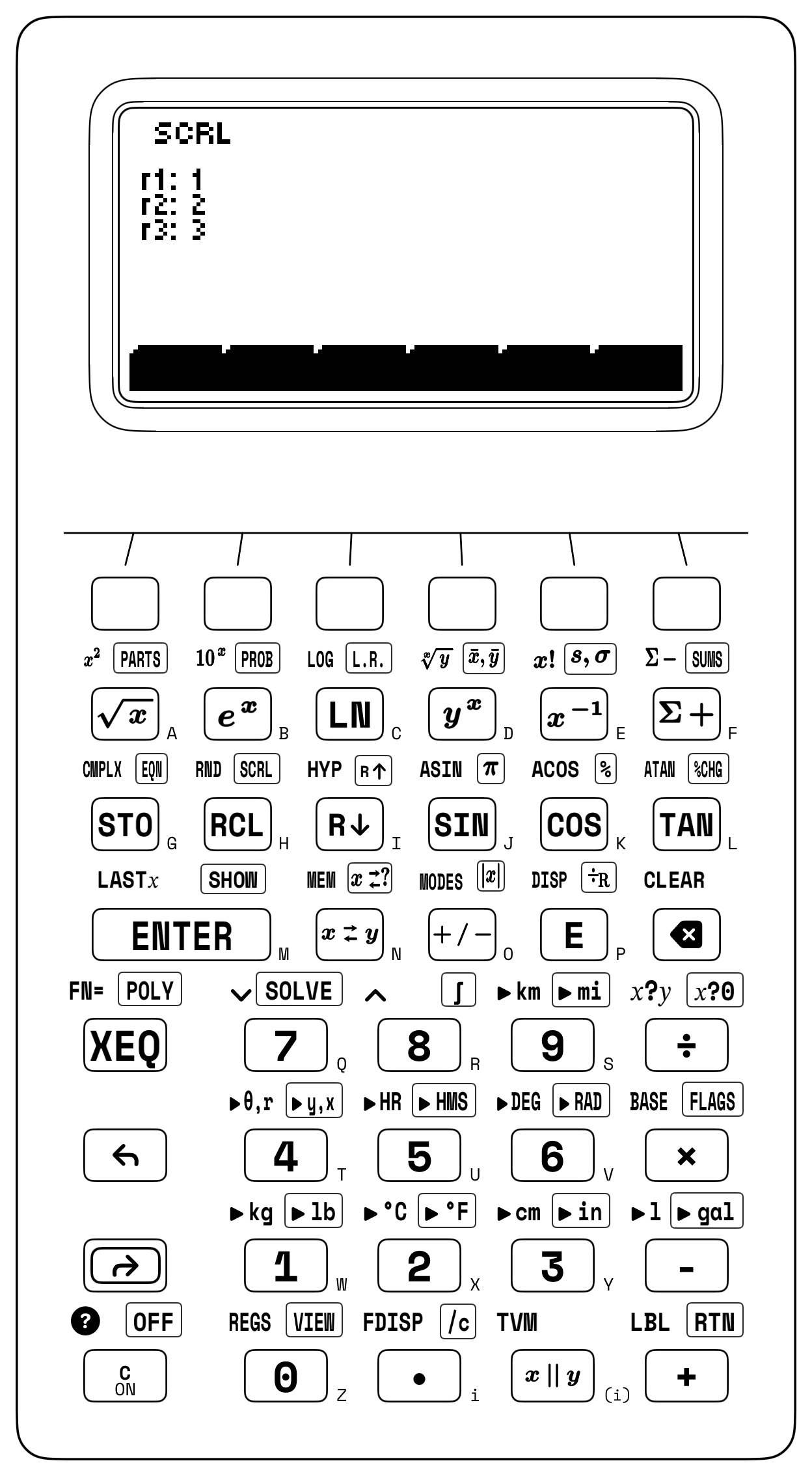
4. Executing ([XEQ]) & Reading All Roots: Pressing [XEQ] while in POLY mode (or any equation variable mode) dispatches to the Cardano–Viète cubic solver (when \(A \ne 0\)) or the quadratic solver (when \(A = 0\) and \(B \ne 0\)). The display presents a multi-line summary of all roots together (r1:, r2:, r3:, Figure 7.2), places the primary root \(r_1\) onto the stack (Register Y = Real, Register X = Imag), and records all roots as (Real, Imag) pairs in the [↰] [REGS] viewer (left-shifted on [0], under STO slots R1–R6 and indirect registers R34–R39).
5. Symbolic Equation Bank ([↱] [EQN]), Function Selection (FN=), & Brent's Root-Finder ([↱] [SOLVE]): When higher-degree or transcendental terms rule out closed-form extraction, press [↱] [EQN] (right-shifted on [STO]), tap NEW, and press a letter (A–Z) to record \(f(x) = \text{LHS} - \text{RHS}\) in RPN using [RCL] + letter, pressing [↱] [EQN] again to save (within the editor, you can also insert LBL/RTN via left/right-shift on [+], step between stored equations with [↰] [↓]/[↰] [↑] on [7]/[8], and scroll long formulas with right-shifted SCRL on [RCL]). Pre-select the equation via FN= (left-shifted on [XEQ]) or select it after pressing [↱] [SOLVE] (right-shifted on [7]), tapping its softkey, and pressing the unknown variable's letter at SOLVE _ (or tapping its variable softkey; typing a value and tapping a variable softkey stores that parameter directly). The calculator prompts (A?, B? \(\to\) value + [ENTER] or [XEQ]) for unassigned parameters, seeds Brent's solver from \(x_0\) (defaulting to \(0\)) to bracket a sign change, and lifts the stack by one level to push \(x^*\) into Register \(X\) (moving the starting seed into \(Y\) and lifting prior \(Y \to Z\) and \(Z \to T\)); storing \(x^*\) and pressing [XEQ] evaluates the residual \(f(x^*)\) in Register \(X\).

7.3.1 Horner's Nested Evaluation & T-Register Flooding

For the fourth-degree polynomial \(P(x) = 4x^4 - 3x^3 + 2x^2 - 5x + 7 = (((4x - 3)x + 2)x - 5)x + 7\) evaluated at \(x_0 = 2.5\), where synthetic division yields \(P(x) = (x - 2.5)(4x^3 + 7x^2 + 19.5x + 43.75) + 116.375\), the four-register stack supports two execution patterns depending on whether \(x_0 = 2.5\) is keyed at each stage or dispensed from Register \(T\). When \(x_0 = 2.5\) is keyed at each stage, the Horner synthetic-division coefficients accumulate sequentially in Register \(X\): \(b_3 = 4(2.5) - 3 = \mathbf{7}\), \(b_2 = 7(2.5) + 2 = \mathbf{19.5}\), \(b_1 = 19.5(2.5) - 5 = \mathbf{43.75}\), and finally the remainder \(b_0 = P(2.5) = 43.75(2.5) + 7 = \mathbf{116.375}\).

To avoid keying \(2.5\) four separate times—or re-typing an irrational evaluation point like \(x \approx 2.718\)—three presses of ENTER fill all four registers \((T, Z, Y, X)\) with \(x_0\) and turn Register \(T\) into an automatic constant dispenser. Every time multiplication consumes the copy of \(x_0\) in Register \(Y\) and drops the stack, Register \(T\) clones a fresh copy of \(x_0 = 2.5\) downward into Register \(Z\), reaching \(\mathbf{116.375}\) without re-typing \(2.5\):

Keystroke	Register T	Register Z	Register Y	Register X	What Happens on the Stack
2.5 [ENTER] [ENTER] [ENTER]	\(2.5\)	\(2.5\)	\(2.5\)	\(2.5\)	Flood stack \((T, Z, Y, X)\) with \(x_0 = 2.5\)
4 [×] 3 [-]	\(2.5\)	\(2.5\)	\(2.5\)	\(7\)	First Horner stage \(b_3 = 4(2.5) - 3 = 7\); \(T\) clones \(2.5\)
[×] 2 [+]	\(2.5\)	\(2.5\)	\(2.5\)	\(19.5\)	Second Horner stage \(b_2 = 7(2.5) + 2 = 19.5\); \(T\) clones \(2.5\)
[×] 5 [-]	\(2.5\)	\(2.5\)	\(2.5\)	\(43.75\)	Third Horner stage \(b_1 = 19.5(2.5) - 5 = 43.75\); \(T\) clones \(2.5\)
[×] 7 [+]	\(2.5\)	\(2.5\)	\(2.5\)	\(116.375\)	Final remainder \(b_0 = P(2.5) = 43.75(2.5) + 7 = \mathbf{116.375}\)

T-register replication also evaluates the rational-logarithmic solar-cell fill factor \(FF = \frac{v_{\text{oc}} - \ln(v_{\text{oc}} + 0.72)}{v_{\text{oc}} + 1}\) at \(v_{\text{oc}} = 25.145\) after entering \(25.145\) only once: flooding the four stack registers with \(v_{\text{oc}}\) supplies one copy for \(\ln(v_{\text{oc}} + 0.72)\), a second waiting copy in Register \(Y\) to subtract that logarithm and form the numerator \(\approx 21.892\), and a third copy replicated from Register \(T\) to form the denominator \(v_{\text{oc}} + 1 = 26.145\) and resolve \(FF \approx \mathbf{0.837}\).

To solve a monic quadratic \(x^2 + 2px + q = 0\) via the single-entry half-linear formula \(r_{1,2} = -p \pm \sqrt{p^2 - q}\) on the stack—such as the coupled-oscillator biquadratic \(u^2 - 10u + 9 = 0\) (\(u = \omega^2\), where \(-p = 5\) and \(q = 9\))—duplicating \(-p = 5\) into Register \(Y\), squaring \(5^2 = 25\), subtracting \(q = 9\), and taking the square root places \(\sqrt{p^2 - q} = 4\) in Register \(X\) with \(-p = 5\) waiting in Register \(Y\). Adding yields the first root \(u_1 = 5 + 4 = \mathbf{9}\) (\(\omega_1 = \mathbf{3}\)) while saving \(\sqrt{p^2 - q} = 4\) in LASTX, so recalling LASTX, doubling (\(8\)), and subtracting yields the second root \(u_2 = 9 - 8 = \mathbf{1}\) (\(\omega_2 = \mathbf{1}\)) without re-typing \(p\) or \(q\).

---

7.3.2 Cardano's Analytical Cubic & Quadratic Solver

On our casus irreducibilis benchmark \((x - 1)(x - 2)(x - 3) = x^3 - 6x^2 + 11x - 6 = 0\) (\(\Delta < 0\)), the POLY softkey sequence proceeds in three steps:

1. Open the POLY workspace (Ax^3 + Bx^2 + Cx + D), and tap the fifth softkey (CLR) if any softkey labels already carry a bullet (•).
2. Key 1 and tap the first softkey A (A• appears); key -6 and tap the second softkey B (B•); key 11 and tap the third softkey C (C•); key -6 and tap the fourth softkey D (D•).
3. Press XEQ.

The solver evaluates Cardano's depressed cubic via complex polar cube-root trisection \(r^{1/3}[\cos(\theta/3) + i\sin(\theta/3)]\) (algebraically equivalent to Viète's cosine trisection when \(\Delta < 0\)), projects the three cube-root branches onto the real axis, and sorts all three real roots in ascending order: the display lists r1: 1, r2: 2, and r3: 3 (Figure 7.2), places the primary root \(r_1 = \mathbf{1}\) in Register \(Y\) (with its imaginary part \(\mathbf{0}\) in Register \(X\)), and stores all three roots across REGS slots R34–R35 (\(r_1 = 1 + 0i\)), R36–R37 (\(r_2 = 2 + 0i\)), and R38–R39 (\(r_3 = 3 + 0i\)). In the positive-discriminant regime (\(\Delta > 0\)), a cubic with complex conjugate roots, as in \(x^3 - x^2 + x - 1 = (x - 1)(x^2 + 1) = 0\), crosses the horizontal axis only once at \(r_1 = 1\), placing \(r_1 = 1 + 0i\) in \((Y, X)\) and storing the pure imaginary conjugate roots \(r_{2,3} = 0 \pm 1i\) in REGS slots R36–R37 and R38–R39.

When a steel bridge joint or aircraft wing root is pulled, compressed, and twisted in three dimensions, rotating a small test cube inside the metal always reveals three mutually perpendicular axes along which sideways shearing forces vanish, leaving only pure tension or compression. Finding those three principal stresses \(\sigma_3 \le \sigma_2 \le \sigma_1\) requires solving a three-real-root cubic (\(\Delta \le 0\)) whose coefficients are the coordinate-independent stress invariants \(I_1, I_2,\) and \(I_3\).

For the 3D principal stress cubic (\(\lambda^3 - 70\lambda^2 + 1175\lambda - 5750 = 0\)) of a structural steel element with tensor invariants \(I_1 = 70\text{ MPa}\), \(I_2 = 1175\text{ MPa}^2\), and \(I_3 = 5750\text{ MPa}^3\), entering \((A = 1,\; B = -70,\; C = 1175,\; D = -5750)\) into the four softkeys and pressing XEQ displays all three stresses together (r1: 10, r2: 11.972, r3: 48.028) and places the minor principal stress \(\sigma_3 = \mathbf{10\text{ MPa}}\) in Register \(Y\) (with \(0\) in Register \(X\)), while the intermediate stress \(\sigma_2 \approx \mathbf{11.972\text{ MPa}}\) and major principal stress \(\sigma_1 \approx \mathbf{48.028\text{ MPa}}\) appear as r2 and r3 (and in REGS slots R36 and R38). Halving the difference between the major and minor principal stresses yields the Tresca maximum shear stress \(\tau_{\max} = \frac{1}{2}(\sigma_1 - \sigma_3) \approx \mathbf{19.014\text{ MPa}}\).

Because any unassigned softkey defaults to 0, depressed cubics and quadratic equations require even fewer entries. On the floating-sphere buoyancy cubic for a solid oak marine buoy of radius \(R = 0.5\text{ m}\) (\(1\text{ m}\) diameter) and specific gravity \(\rho_s/\rho_w = 0.65\), balancing submerged spherical-cap volume against displaced water weight yields \(h^3 - 3Rh^2 + 4(\rho_s/\rho_w)R^3 = h^3 - 1.5h^2 + 0.325 = 0\), which has no linear \(h\) term. After tapping CLR, you enter only \(A = 1\), \(B = -1.5\), and \(D = 0.325\) on the softkeys (with softkey C left untouched at its default of 0) and press XEQ to read the physical waterline draft \(h \approx \mathbf{0.601\text{ m}}\) as r2 (\(\approx 60.1\%\) submerged), while the algebraic companion roots \(\approx -0.412\text{ m}\) and \(\approx 1.311\text{ m}\) lie outside the physical sphere \([0, 1\text{ m}]\).

On the inverse ballistic quadratic \(360.367 u^2 - 1200u + 510.367 \approx 0\) for an elevated target at range \(x = 1,200\text{ m}\) and height \(y = 150\text{ m}\) (\(v_0 = 140\text{ m/s}, g = 9.81\text{ m/s}^2\)), leaving A at its 0 default and assigning \(B = 360.367\), \(C = -1200\), and \(D = 510.367\) extracts both roots upon pressing XEQ. Taking the arctangent of the two positive slope roots returns both the low direct-fire angle \(\theta_1 \approx \mathbf{26.59^\circ}\) and the high plunging mortar arc \(\theta_2 \approx \mathbf{70.535^\circ}\).

---

7.3.3 Taming Transcendental Equations by Bracketed Iteration

A comparison of the iterative equation solver (EQN and SOLVE) with the closed-form polynomial solver (POLY) on two physical cubics contrasts bracketed root-finding with analytical extraction. On Newton's cubic benchmark \(x^3 - 2x - 5 = 0\), hand-evaluating Cardano's formula requires the sum of two nested cube roots \(\sqrt[3]{\frac{5}{2} + \sqrt{\frac{643}{108}}} + \sqrt[3]{\frac{5}{2} - \sqrt{\frac{643}{108}}}\). Entering the residual \(f(x) = (x^2 - 2)x - 5\) in Horner nested form and storing the starting seed \(x_0 = 2\) (where \(f(2) = -1 < 0\) and \(f(3) = +16 > 0\)) expands an outward sign-change bracket around \(x_0 = 2\) and converges to \(x^* \approx \mathbf{2.095}\) in Register \(X\) with a machine-zero residual \(|f(x^*)| < 10^{-15}\).

For carbon dioxide (\(\text{CO}_2\), \(a = 3.59\text{ L}^2\cdot\text{atm/mol}^2\), \(b = 0.043\text{ L/mol}\)) compressed to \(P = 50\text{ atm}\) at \(T = 300\text{ K}\) (\(RT = 24.618\text{ L}\cdot\text{atm/mol}\)), the van der Waals real-gas equation of state \(\left(P + \frac{a}{V^2}\right)(V - b) = RT\) clears the \(V^2\) denominator to form the expanded cubic \(50V^3 - 26.768V^2 + 3.59V - 0.154 = 0\). Both the cubic polynomial solver and Brent's root-finder (seeded at the ideal-gas volume \(V_{\text{ideal}} = RT/P \approx 0.492\text{ L/mol}\) on the unexpanded van der Waals residual) find the real molar volume \(V_m \approx \mathbf{0.359\text{ L/mol}}\)—\(27\%\) smaller in molar volume (\(37\%\) denser) than the ideal-gas estimate, corresponding to a compressibility factor \(Z = P V_m / RT \approx \mathbf{0.729}\).

On coupled transcendental conservation laws, Brent's solver resolves the unknowns from their equation residuals. For Kepler's elliptical orbital anomaly \(E - e\sin E - M = 0\) on an Earth-observation satellite with orbital eccentricity \(e = 0.25\) at mean anomaly \(M = 1.2\text{ rad}\) in radian mode, \(|\sin E| \le 1\) guarantees that the physical root lies inside \([M - e,\; M + e] = [0.95,\; 1.45]\text{ rad}\); seeding \(E_0 = 1.2\) converges to \(E^* \approx \mathbf{1.448\text{ rad}}\) (\(\approx 82.971^\circ\)) in five iterations.

In fluid pipelines and nonlinear circuits, bracketed iteration isolates implicit operating points without divergence. Evaluating the Colebrook–White turbulent pipe friction residual \(g(f) = \frac{1}{\sqrt{f}} + 2\log_{10}\!\left(\frac{\varepsilon/D}{3.7} + \frac{2.51}{\text{Re}\sqrt{f}}\right) = 0\) at Reynolds number \(\text{Re} = 100,000\) and relative roughness \(\varepsilon/D = 0.001\) by seeding \(f_0 = 0.02\) inside the physical Moody turbulent regime \([0.008, 0.08]\) lifts \(0.02\) into Register \(Y\) and converges to \(f^* \approx \mathbf{0.022}\) in Register \(X\).

On the silicon diode load-line residual \(f(V) = 5 - 10^{-9}(e^{V/V_T} - 1) - V = 0\) (\(V_s = 5\text{ V}\), \(I_s R = 10^{-9}\text{ V}\), \(V_T \approx 0.026\text{ V}\))—where an unguarded Newton step from \(V_0 = 0\text{ V}\) shoots along the flat tangent to \(+5\text{ V}\) (\(e^{5 / V_T} \approx 10^{84}\))—a starting guess near the silicon turn-on knee at \(V_0 = 0.65\text{ V}\) converges safely to \(V_D^* \approx \mathbf{0.577\text{ V}}\) (\(I_D \approx 4.423\text{ mA}\)).

When \(Q = 20\text{ m}^3/\text{s}\) (\(Q^2 = 400\)) of floodwater rushes through a trapezoidal concrete spillway of bottom width \(b = 3\text{ m}\) and side slopes \(z = 2\), the critical depth \(y_c\) (\(\text{Fr} = 1\)) crosses the degree-4 radical barrier to form the sixth-degree polynomial \(f(y) = 400(3 + 4y) - 9.81(3y + 2y^2)^3 = 0\), where seeding at \(y_0 = 1\text{ m}\) converges to \(y_c^* \approx \mathbf{1.251\text{ m}}\).

Bracketed root-finding also selects distinct physical branches when a conservation law admits multiple solutions on opposite sides of a singularity or throat. In compressible gas dynamics, the De Laval rocket nozzle area–Mach relation \(\frac{1}{M}\left(\frac{1 + 0.2M^2}{1.2}\right)^3 - 2.5 = 0\) for an expansion area ratio \(A/A^* = 2.5\) and specific-heat ratio \(\gamma = 1.4\) admits two physical flow regimes separated by the \(M^* = 1\) sonic throat. Seeding above the throat (\(M_0 = 2.5\) in \([1.05, 4]\)) locks Brent's solver onto the accelerating supersonic exhaust branch \(M_{\text{sup}} \approx \mathbf{2.443}\); seeding below the throat (\(M_0 = 0.2\) in \([0.05, 0.95]\)) isolates the decelerating subsonic venturi diffuser branch \(M_{\text{sub}} \approx \mathbf{0.24}\).

7.3.4 Practical Root-Finding Strategy & Residual Verification

To verify how a single Newton–Raphson step \(E_1 = E_0 - \frac{E_0 - e\sin E_0 - M}{1 - e\cos E_0}\) refines an orbital anomaly estimate on the four-register stack, flood the stack \((T, Z, Y, X)\) with the upper bracket endpoint \(E_0 = M + e = 1.45\text{ rad}\) in radian mode. Evaluating \(0.25\sin(1.45)\) and subtracting from the waiting copy of \(E_0\) in Register \(Y\) followed by \(M = 1.2\) isolates the residual \(f(1.45) \approx 1.822 \times 10^{-3}\text{ rad}\) in Register \(X\); dividing by the slope \(f'(1.45) = 1 - 0.25\cos(1.45) \approx 0.97\) to form the step \(\Delta E \approx 1.878 \times 10^{-3}\text{ rad}\) and subtracting from the copy of \(E_0\) dispensed by Register \(T\) reaches \(E_1 \approx \mathbf{1.448\text{ rad}}\) without re-entering \(E_0\). When an equation is already a contraction mapping \(x = g(x)\) (\(|g'(x^*)| < 1\)), applying \(g\) repeatedly to Register \(X\)—pressing cosine in radian mode to watch \(x_{n+1} = \cos(x_n)\) spiral into the Dottie fixed point \(x^* \approx \mathbf{0.739\text{ rad}}\), or flooding Register \(T\) with \(c = 6\) and repeating addition and square root to watch \(\sqrt{6 + \sqrt{6 + \dots}}\) converge to \(\mathbf{3}\)—visualizes fixed-point convergence before handing stiffer residuals \(g(x) - x = 0\) to Brent's solver.

After the root-finder terminates, storing the converged root estimate \(x^*\) into the equation's target variable and pressing XEQ to evaluate the stored equation performs the residual audit \(f(x^*)\), where a genuine root yields \(|f(x^*)| \le 10^{-12}\) while an accidental vertical asymptote or pole exposes itself with \(|f(x^*)| \gg 1\).

Three algebraic habits reinforce polynomial and transcendental root-finding. First, when POLY displays r1, r2, r3 of \(Ax^3 + Bx^2 + Cx + D = 0\) (and stores their real and imaginary parts in REGS STO slots R34–R39), Viète's identities provide an immediate checksum: summing the three real parts equals \(-B/A\) (\(10 + 11.972 + 48.028 = \mathbf{70}\)), multiplying three real roots equals \(-D/A\) (\(\mathbf{5750}\)), and when \(r_{2,3} = \alpha \pm i\beta\) are complex conjugates, converting \((\beta, \alpha)\) to polar form extracts \(|r_2| = \sqrt{\alpha^2 + \beta^2}\) so \(r_1 |r_2|^2 = r_1(\alpha^2 + \beta^2) = -D/A\). Second, when an equation has multiple roots across physical regimes—such as subsonic versus supersonic Mach branches across the \(M^* = 1\) throat—an initial seed \(x_0\) inside the target regime (\(M_0 = 0.2\) or \(M_0 = 2.5\)) locks Brent's solver inside that branch. Third, storing a known root \(r_1\) in Variable \(A\) (deflating in order \(|r_1| \le |r_2|\)) and dividing the residual in EQN by \((X - A)\) forms \(g(x) = \frac{f(x)}{x - r_1}\) so a subsequent solver pass cannot fall back into \(r_1\).

7.3.5 Try It on the Stack

1. Standard Atmosphere Pressure Polynomial via \(T\)-Flooding: Flood \((T, Z, Y, X)\) with altitude \(h = 8.435\text{ km}\) and evaluate \(P(h) = ((-0.025h + 0.95)h - 12)h + 101.325\text{ kPa}\) without re-typing \(h\). (Verified Register \(X\) result: \(P \approx \mathbf{52.693\text{ kPa}}\).)
2. Depressed Cubic & Viète Root-Power Sum in POLY: Clear POLY slots to \(0\), enter \(A = 1\), \(C = -7\), and \(D = 6\) (leaving \(B\) at \(0\)) for \(x^3 - 7x + 6 = 0\), execute, and verify \(r_1^2 + r_2^2 + r_3^2 = (B/A)^2 - 2(C/A) = \mathbf{14}\). (Verified roots: \(r_1 = \mathbf{-3}\), \(r_2 = \mathbf{1}\), \(r_3 = \mathbf{2}\), with \((-3)^2 + 1^2 + 2^2 = \mathbf{14}\).)
3. Quadratic Golden-Ratio Root Extraction: In POLY, clear slots so \(A = 0\), assign \(B = 1\), \(C = -1\), and \(D = -1\) for \(x^2 - x - 1 = 0\), and execute to obtain both roots. (Verified roots: \(r_1 \approx \mathbf{-0.618}\) and \(r_2 \approx \mathbf{1.618}\).)