Chapter 5: Complex Numbers, Euler's Identity & Alternating-Current Phasors
In August 1893, at the International Electrical Congress in Chicago, Charles Proteus Steinmetz presented a paper that resolved the central mathematical bottleneck of the electrical age: "Complex Quantities and Their Use in Electrical Engineering" (Steinmetz, 1893). Whereas a static survey triangle sits fixed in a two-dimensional plane, alternating-current (AC) power grids, mechanical vibrations, and radio waves spin continuously in time. As high-voltage AC transmission lines expanded across long distances, engineers faced a formidable barrier: while direct-current (DC) networks obeyed scalar Ohm's law (\(V = I \cdot R\)), alternating current oscillating at frequency \(f\) shifted voltage and current out of phase by \(\pm 90^\circ\) across inductive coils and capacitive plates, turning every multi-branch circuit calculation into a system of coupled linear differential equations.
Steinmetz recognized that the key to turning AC calculus back into simple algebra had been hiding for centuries inside the square root of negative one, \(\sqrt{-1}\). Because the square of any non-zero real number is positive (\(+3 \times +3 = +9\) and \(-3 \times -3 = +9\)), no point on the one-dimensional real number line has a negative square, leading René Descartes in 1637 to dismiss such roots as "imaginary" (Descartes, 1637). Even when sixteenth-century algebraists solved the real cubic equation \(x^3 = 15x + 4\) (whose positive real root is \(x = 4\), since \(4^3 = 64 = 15(4) + 4\)), the closed-form cubic formula forced the calculation through conjugate radicals containing \(\sqrt{-121} = 11\sqrt{-1}\):
To reach a real root from real coefficients required stepping off the real line into a perpendicular dimension—and as Steinmetz demonstrated in Chicago, that two-dimensional plane is the natural coordinate system of every oscillating wave and alternating current.
5.1 Orthogonal Rotation in the Complex Plane & Euler's Identity
The perpendicular direction of \(\sqrt{-1}\) follows from the geometry of multiplication along the real line, where multiplying by \(-1\) acts as a continuous rotation in the plane. For a unit vector at the origin \(0\) directed along the positive real axis toward \(+1\) (\(0^\circ\)), multiplying by \(-1\) preserves its unit length while rotating its heading by \(180^\circ\) to point along the negative real axis toward \(-1\). Multiplying by \(-1\) a second time rotates the vector by a further \(180^\circ\), completing a \(360^\circ\) revolution back to \(+1\):
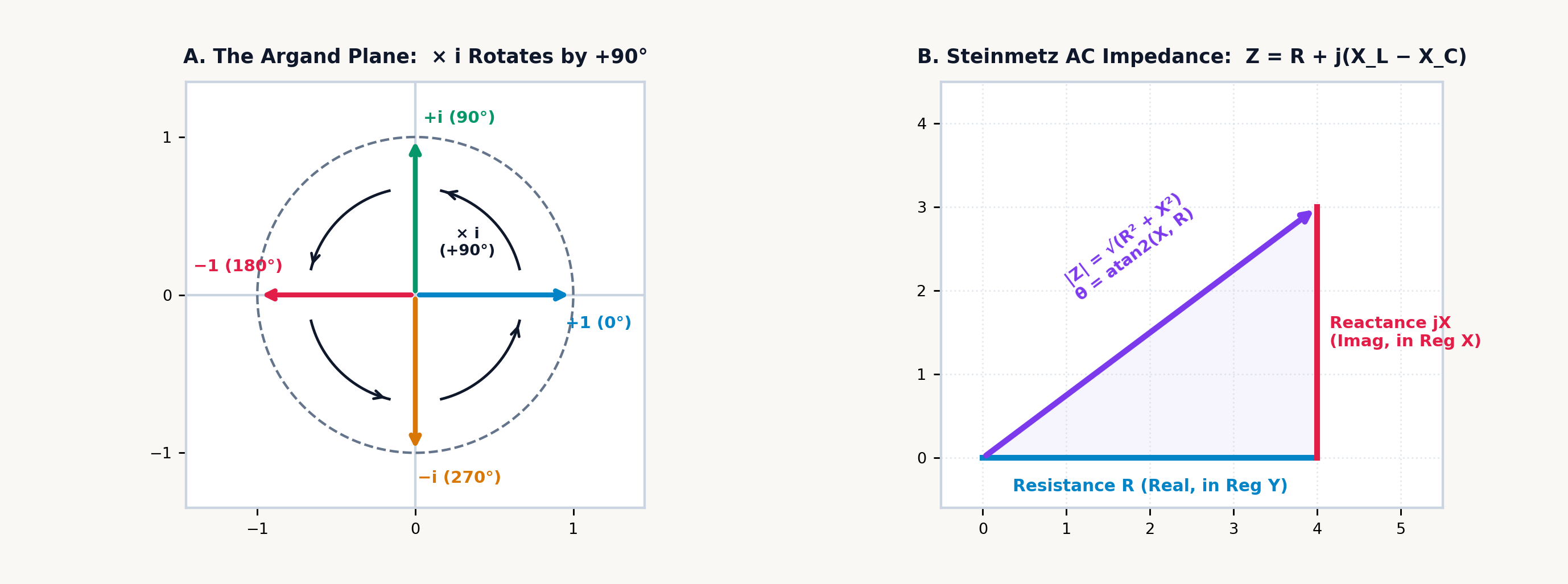
Multiplication by \(-1\) acts as a \(180^\circ\) half-turn, which defines \(i = \sqrt{-1}\) as a \(90^\circ\) counterclockwise quarter-turn. Starting at \(i^0 = +1\) along the positive real axis at \(0^\circ\), a single multiplication by \(i\) rotates the vector \(90^\circ\) counterclockwise onto the perpendicular vertical axis at \(+i\). A second multiplication (\(i \times i = i^2 = -1\)) rotates the vector by a second \(90^\circ\) quarter-turn (\(90^\circ + 90^\circ = 180^\circ\)) onto the negative real axis at \(-1\); two \(90^\circ\) rotations compose into a \(180^\circ\) reversal, which is the geometric meaning of \(i^2 = -1\). A third quarter-turn (\(i^3 = -i\)) directs the vector along the negative vertical axis at \(270^\circ\), and a fourth quarter-turn (\(i^4 = +1\)) completes the \(360^\circ\) cycle back to \(+1\).
A complex number \(z = a + bi\) therefore specifies a point or vector in the two-dimensional Complex Plane (Argand Diagram) through a displacement of \(a\) units along the horizontal Real axis and \(b\) units along the perpendicular vertical Imaginary axis (Figure 5.1).
5.1.1 Conjugates, Rotations, and Overflow-Safe Division
Because a complex number \(z = a + bi\) is an ordered pair \((a, b)\) on a two-dimensional plane, every arithmetic operation has a direct geometric meaning in terms of vector translation, scaling, and rotation.
Under complex addition and subtraction, two complex vectors \(z_1 = a + bi\) and \(z_2 = c + di\) combine by head-to-tail translation, summing their horizontal components and vertical components independently:
Under complex multiplication, expanding the binomial product \((a + bi)(c + di)\) with \(i^2 = -1\) groups the two real terms \(ac\) and \(i^2 bd = -bd\) along the horizontal axis and the two cross-terms \(adi\) and \(bci\) along the vertical axis, so \((3 + 4i)(1 - 2i) = (3 + 8) + (-6 + 4)i = \mathbf{11 - 2i}\):
Complex reciprocals and division rely on reflection across the real axis. Every complex number \(z = c + di\) has a reflection twin called its complex conjugate, \(z^* = c - di\), formed by negating the imaginary component. If \(z\) lies at angle \(+\theta\) relative to the positive real axis, \(z^*\) lies at \(-\theta\); multiplying \(z\) by its conjugate \(z^*\) cancels their opposite angles (\(\theta - \theta = 0^\circ\)) and yields the nonnegative real squared modulus \(|z|^2 = c^2 + d^2\):
For a complex quotient \(\frac{a + bi}{c + di}\), multiplying numerator and denominator by the denominator's conjugate \(c - di\) reduces the denominator to the real scalar \(c^2 + d^2\):
In finite-precision IEEE-754 floating-point arithmetic, unscaled evaluation of the algebraic quotient \(\frac{(ac+bd) + i(bc-ad)}{c^2+d^2}\) fails whenever \(|c|\) or \(|d|\) exceeds the square root of the overflow threshold (\(\sqrt{\Omega_{\max}} \approx 1.34 \times 10^{154}\)) or falls below the square root of the normal underflow threshold (\(\approx 1.49 \times 10^{-154}\)). Even when the quotient \(\frac{3 \times 10^{200} + 4 \times 10^{200}i}{3 \times 10^{200} + 4 \times 10^{200}i} = 1 + 0i\) equals unity, squaring \(c^2 + d^2 = 25 \times 10^{400}\) overflows an unscaled divider.
To prevent premature overflow above \(10^{154}\) or underflow below \(10^{-154}\), complex division and reciprocals on the SC-32 pivot on the larger denominator component:
By forming the smaller-over-larger ratio \(r = d/c\) or \(r = c/d\) so that \(|r| \le 1\) (Robert L. Smith's 1962 scaling algorithm), every intermediate product remains bounded within the exponent range of the operands. Dividing \((3 + 4i) \times 10^{200}\) by \((3 - 4i) \times 10^{200}\) evaluates to \(-0.28 + 0.96i\) without intermediate exponent overflow.
For any nonzero \(z = a + bi \ne 0\), the complex square root avoids subtractive cancellation in the half-angle radical \(\sqrt{\frac{|z| + a}{2}}\) when \(a < 0\) and \(|b| \ll |a|\) by evaluating the larger root component first from the scaled hypotenuse \(|z| = \operatorname{hypot}(a, b)\) and recovering the smaller component by division (where the branch-cut sign \(\sigma(b) = +1\) for \(b \ge 0\) and \(-1\) for \(b < 0\) maps the negative real axis \(b = 0,\; a < 0\) onto the positive imaginary axis \(+i\sqrt{|a|}\)):
5.1.2 Complex Eigenvalues in Damped Springs and Skyscrapers
This orthogonal separation between the real and imaginary axes characterizes linear damped oscillators across mechanical and structural engineering, from vehicle suspension struts to tuned mass dampers in tall buildings.
When a mass \(m\) coupled to a spring of stiffness \(k\) and a viscous damper of coefficient \(c\) is displaced from equilibrium, the balance of forces gives the homogeneous differential equation \(m\ddot{x} + c\dot{x} + kx = 0\). Substituting an exponential trial solution \(x(t) = e^{\lambda t}\) produces the quadratic characteristic equation \(m\lambda^2 + c\lambda + k = 0\), whose roots are the system's eigenvalues:
Whenever the restoring stiffness exceeds the damping threshold (\(k/m > (c/2m)^2\)), the discriminant is negative and the eigenvalues form a complex conjugate pair \(\lambda = -\alpha \pm i\omega_d\). The two axes of the complex plane separate the two physical processes acting in the oscillator. Along the real axis, the attenuation rate \(-\alpha = -c/(2m)\) measures irreversible energy dissipation: viscous fluid forced through the damper orifices resists motion in phase with velocity and converts mechanical kinetic energy into heat, so the oscillation envelope decays exponentially as \(e^{-\alpha t}\).
Along the vertical Imaginary axis, the damped natural frequency \(\pm i\omega_d\) measures lossless quadrature energy exchange: the spring and mass dissipate no heat, exchanging kinetic energy in the moving mass (\(\frac{1}{2}mv^2\), which peaks at the equilibrium crossing) with potential energy in the strained spring (\(\frac{1}{2}kx^2\), which peaks at the turning points) \(90^\circ\) out of phase at angular frequency \(\omega_d = \sqrt{k/m - \alpha^2}\). In the undamped limit (\(c \to 0\)), the real part \(-\alpha\) vanishes, the eigenvalues lie on the imaginary axis (\(\lambda = \pm i\sqrt{k/m}\)), and the oscillation persists at constant amplitude. At the critical damping threshold \(c_{\text{crit}} = 2\sqrt{mk}\), the imaginary part \(\omega_d\) vanishes and the displaced mass returns to equilibrium without oscillation.
5.1.3 Euler's Formula and the Three-Phase Roots of Unity
For an imaginary argument \(z = i\theta\), the exponential function \(e^z\) connects continuous exponential scaling along the real line (\(e^x\)) to circular rotation around the unit circle (\(\cos\theta, \sin\theta\)) through Euler's formula:
Exponential functions and circular trigonometric functions are orthogonal cross-sections of a single analytic function \(e^z\) in the complex plane: along the real axis \(e^z\) scales exponentially in magnitude, and along the imaginary axis \(e^z\) rotates at unit radius around the origin.
The unit-circle trajectory of \(e^{i\theta}\) follows independently from differential kinematics and from power-series expansion. In differential kinematics, when a state variable \(z(t)\) evolves at a real growth rate \(k\), its velocity vector \(dz/dt = k \cdot z\) is collinear with the position vector \(z\), driving the trajectory radially outward or inward along a straight ray from the origin. Replacing the real rate \(k\) with the imaginary rate \(i\omega\) gives the differential equation:
Because multiplication by \(i\) rotates any complex vector by \(90^\circ\) counterclockwise, the velocity vector \(dz/dt\) of \(z(t) = e^{i\omega t}\) is at every instant perpendicular (\(90^\circ\)) to the radius vector \(z(t)\), identical to the tangential velocity of uniform circular motion. Because a velocity orthogonal to the radius performs zero radial work and changes the radial distance at rate \(\frac{d}{dt}|z|^2 = 0\), the modulus remains invariant at \(|e^{i\theta}| = 1\) for all real \(\theta\), while the point traces the unit circle with horizontal projection \(\cos\theta\) and vertical projection \(i\sin\theta\).
Algebraically, substituting \(x = i\theta\) into the Maclaurin series for \(e^x\) and reducing the powers \(i^2 = -1\), \(i^3 = -i\), and \(i^4 = +1\) separates the real even-power terms from the imaginary odd-power terms to recover the Maclaurin series for cosine and sine:
At a half-revolution \(\theta = \pi\text{ radians}\) (\(180^\circ\)), where \(\cos\pi = -1\) and \(\sin\pi = 0\), Euler's formula gives \(e^{i\pi} = -1\), or in homogeneous form:
which links the additive identity \(0\), the multiplicative identity \(1\), the circle constant \(\pi\), the base of natural logarithms \(e\), and the imaginary unit \(i\). At the principal quarter-turn \(\theta = \pi/2\), where \(i = e^{i\pi/2}\), raising \(i\) to the \(i\)-th power yields the principal real value \(i^i = \left(e^{i\pi/2}\right)^i = e^{i^2 \pi/2} = e^{-\pi/2} \approx 0.208\) (with general multivalued branches \(e^{-(\pi/2 + 2\pi k)}\) for \(k \in \mathbb{Z}\)).
By Euler's formula, any nonzero complex number \(z = x + iy\) can be expressed in polar form through its Euclidean modulus \(r = |z| = \sqrt{x^2 + y^2}\) and its principal argument \(\theta = \operatorname{atan2}(y, x)\):
Whereas two-dimensional vector conversions place the horizontal coordinate \(x\) and radial magnitude \(r\) in Register \(X\), algebraic complex arithmetic writes a complex number in top-to-bottom reading order as \(z = a + bi\), pairing the real projection \(a = \operatorname{Re}(z)\) in the upper register of a two-line pair (\(Y\) or \(T\)) and the imaginary projection \(b = \operatorname{Im}(z)\) in the lower register (\(X\) or \(Z\))—so the lower pair is swapped whenever converting between a complex number \((Y = a,\; X = b)\) and the polar vector \((Y = b,\; X = a) \leftrightarrow (Y = \theta,\; X = r)\).
In polar form \(z = r e^{i\theta}\), multiplication, division, and exponentiation follow from the laws of exponents. Multiplying two complex numbers \(z_1 z_2 = (r_1 e^{i\theta_1})(r_2 e^{i\theta_2}) = (r_1 r_2) e^{i(\theta_1 + \theta_2)}\) multiplies their moduli and adds their phase angles; dividing two complex numbers \(z_1 / z_2 = (r_1 / r_2) e^{i(\theta_1 - \theta_2)}\) divides their moduli and subtracts their phase angles. Raising \(z = r e^{i\theta}\) to the \(n\)-th power yields de Moivre's theorem, \((r e^{i\theta})^n = r^n e^{in\theta}\):
Geometrically, raising a complex number to the \(n\)-th power raises its modulus to \(r^n\) while multiplying its argument by \(n\). Inverting de Moivre's relation to extract an \(n\)-th root \(\sqrt[n]{z}\) explains why an \(n\)-th degree polynomial equation has \(n\) roots in the complex plane. Because adding integer multiples of a full revolution \(2k\pi\) (\(360^\circ k\)) leaves a complex number unchanged (\(\theta + 2k\pi\)), dividing the angle by \(n\) produces \(n\) distinct roots spaced at equal angular intervals of \(2\pi/n\) around a circle of radius \(r^{1/n}\):
Even the square root of \(i\) (\(\sqrt{i}\)) requires no new class of numbers outside the complex plane: because \(i = 1\angle 90^\circ\) has modulus \(1\) and argument \(90^\circ\), its principal square root has modulus \(\sqrt{1} = 1\) and half the angle, \(45^\circ\) (\(\pi/4\text{ rad}\)), which lies in the complex plane at \(\cos 45^\circ + i\sin 45^\circ = \frac{\sqrt{2}}{2} + i\frac{\sqrt{2}}{2} \approx 0.707 + 0.707i\).
On the real line, the cubic equation \(z^3 = 1\) has only the single root \(1\) (and \(z^3 = -8\) has only the real root \(-2\) alongside the complex conjugate roots \(1 \pm i\sqrt{3}\)). In the complex plane, the three cube roots of unity (\(z^3 = 1 = e^{i\cdot 2k\pi}\)) lie \(360^\circ / 3 = 120^\circ\) apart at the vertices of an equilateral triangle inscribed in the unit circle:
Because those three unit vectors are spaced symmetrically at \(0^\circ\), \(120^\circ\), and \(240^\circ\), their vector sum vanishes (\(1 + a + a^2 = 0\)). This \(120^\circ\) three-phase symmetry is the operating principle of polyphase AC power transmission: in a balanced three-phase network with phase currents displaced by \(0^\circ, 120^\circ,\) and \(240^\circ\), the instantaneous return currents sum to \(1 + a + a^2 = 0\) at the neutral node, allowing three conductors to transmit polyphase power without a fourth return wire.
5.1.4 Principal Branch Cuts and Conformal Airfoil Mapping
Euler's exponential relations extend the circular trigonometric functions analytically to arbitrary complex arguments \(z = x + iy\). For a real angle \(x\), \(\sin x\) and \(\cos x\) are bounded within \([-1, +1]\); combining \(e^{ix} = \cos x + i\sin x\) and \(e^{-ix} = \cos x - i\sin x\) defines cosine and sine across the entire complex plane:
When a complex argument \(z = x + iy\) is evaluated, multiplying the imaginary term \(iy\) by \(i\) inside \(e^{\pm i(x+iy)} = e^{\mp y}e^{\pm ix}\) converts the vertical coordinate \(y\) into real exponential scaling factors \(\frac{e^y + e^{-y}}{2}\) and \(\frac{e^y - e^{-y}}{2}\):
Even when \(e^{|y|}\) drives the magnitudes of \(\sin z\) and \(\cos z\) well past \([-1, +1]\), analytic continuation preserves the Pythagorean identity \(\sin^2 z + \cos^2 z = 1\) across the complex plane. For multivalued inverse and fractional-power functions—such as the complex natural logarithm \(\operatorname{Ln}(\mathbf{z}) = \ln|\mathbf{z}| + i\operatorname{Arg}(\mathbf{z})\), the complex square root \(\sqrt{\mathbf{z}} = \sqrt{|\mathbf{z}|}\,e^{i\operatorname{Arg}(\mathbf{z})/2}\), and general complex powers \(\mathbf{z}^{\mathbf{w}} = e^{\mathbf{w}\operatorname{Ln}(\mathbf{z})}\)—the SC-32 places a principal branch cut along the negative real axis \((-\infty, 0)\) just as cartographers place the International Date Line along the \(180^\circ\) meridian so every point has one unambiguous principal angle \(\operatorname{Arg}(\mathbf{z}) \in (-\pi, \pi]\).
This convention guarantees that the complex square root always maps into the closed right half-plane \(\operatorname{Re}(\sqrt{\mathbf{z}}) \ge 0\) (with \(\sqrt{-4 + 0i} = 0 + 2i\) on the upper boundary of the cut, and \(\operatorname{Ln}(-5 + 0i) = \ln 5 + i\pi \approx 1.609 + 3.142i\)), while a Nyquist contour crossing the negative real axis \((-\infty, 0)\) exhibits a \(2\pi\) phase transition between \(+\pi\) and \(-\pi\).
Holomorphic complex functions also define conformal mappings: at every point where \(f'(z) \ne 0\), a complex mapping \(w = f(z)\) acts like an angle-preserving mathematical lens that transforms solutions of Laplace's equation (\(\nabla^2\phi = 0\)) around a simple shape into exact solutions around a complex shape. Evaluating the sum of a complex coordinate \(z\) on an offset circle (passing through the critical point \(z = +c\) and enclosing \(z = -c\)) and its scaled reciprocal \(c^2/z\) defines the Joukowsky airfoil transformation:
This rational complex map (\(\mathbf{z} + c^2 \cdot \frac{1}{\mathbf{z}}\)) transforms the offset circle into an airfoil profile through three geometric effects: at the critical point \(z = +c\), where the derivative \(d\zeta/dz = 1 - c^2/z^2\) vanishes, the smooth circular boundary folds into a sharp trailing edge at \(\zeta = +2c\); on the opposite side of the circle extending slightly beyond \(z = -c\), the boundary rounds into a blunt leading edge; and displacing the circle's center slightly above the real axis introduces camber along the chord line. Because \(\zeta = z + c^2/z\) is conformal everywhere exterior to the circle, it maps the potential-flow streamlines around a spinning cylinder onto the airflow around the cambered wing: requiring smooth flow off the sharp trailing edge fixes the wing's aerodynamic vortex circulation \(\Gamma\) (the line integral of tangential velocity around the profile), which interacts with the freestream air density \(\rho_\infty\) and freestream airspeed \(V_\infty\) to generate aerodynamic lift per unit wingspan \(L' = \rho_\infty V_\infty \Gamma\) under the Kutta–Joukowsky Lift Theorem.
5.2 Alternating-Current Phasors, Resonance & Wave Reflection
In an alternating-current circuit operating at frequency \(f = 60\text{ Hz}\) (angular frequency \(\omega = 2\pi f\)), inductors and capacitors displace voltage and current by \(\pm 90^\circ\). Track the instantaneous charge \(q(t)\) stored on a capacitor's plates as current \(i(t) = \frac{dq}{dt}\) sloshes back and forth through a series loop of inductance \(L\), resistance \(R\), and capacitance \(C\) driven by an alternating source of peak voltage \(V_0\) and initial phase angle \(\phi\). In the resistor, Ohm's law produces a voltage drop \(R i = R\frac{dq}{dt}\) directly in phase with the current. In the inductor (such as a transformer winding or motor coil), Faraday's law induces a voltage proportional to the current slew rate, \(v_L(t) = L \frac{di}{dt} = L\frac{d^2 q}{dt^2}\); because \(\frac{d}{dt}\sin(\omega t) = \omega\cos(\omega t) = \omega\sin(\omega t + 90^\circ)\), inductor voltage peaks \(90^\circ\) ahead of current. In the capacitor (such as parallel dielectric plates or underground cable insulation), the voltage across the plates is proportional to the accumulated charge, \(v_C(t) = \frac{1}{C}q(t)\), so capacitor voltage lags \(90^\circ\) behind charging current \(i_C = C\frac{dv_C}{dt}\). Summing those three voltage drops around the loop via Kirchhoff's voltage law yields a second-order linear differential equation with sinusoidal forcing:
Each passive element in that loop mirrors a mechanical counterpart: \(L\frac{d^2 q}{dt^2}\) acts like magnetic inertia opposing any sudden change in current (\(d^2q/dt^2\)), \(R\frac{dq}{dt}\) acts like viscous friction dissipating heat in proportion to current velocity (\(dq/dt\)), and \(\frac{1}{C}q\) acts like an elastic spring whose restoring voltage grows with displaced charge \(q\). Steinmetz's 1893 insight was that because multiplication by \(j = \sqrt{-1}\) rotates a vector by \(+90^\circ\) in the complex plane, Euler's complex exponential \(e^{j\omega t}\) turns time differentiation into algebraic multiplication by \(j\omega\), converting that entire differential equation into one line of complex algebra.
5.2.1 Rotating Phasors and the Complex Impedance Plane
In a linear AC network driven at a single angular frequency \(\omega\), every steady-state voltage and current oscillates at that same angular frequency \(\omega\). To avoid carrying explicit \(\cos(\omega t + \theta)\) time functions through differential equations, Steinmetz represented each sinusoid by a complex number—a phasor—scaled by its root-mean-square amplitude (\(|\mathbf{V}| = V_0/\sqrt{2}\), eliminating the factor of \(\frac{1}{2}\) so AC power laws \(P = |\mathbf{I}|^2 R\) and \(\mathbf{S} = \mathbf{V}\mathbf{I}^*\) match DC Ohm's and Joule's laws) and initial phase angle relative to a common reference.
When a rotating complex exponential \(e^{j\omega t}\) is differentiated with respect to time (where electrical engineering denotes the imaginary unit by \(j = \sqrt{-1}\) to reserve \(i\) for electrical current), the phasor is multiplied by \(j\omega\):
Time differentiation becomes algebraic multiplication by \(j\omega\) (a \(+90^\circ\) rotation scaled by \(\omega\)), while time integration becomes division by \(j\omega\) (a \(-90^\circ\) rotation, since \(1/j = -j\)).
Under this phasor transformation, the three passive circuit elements map onto the axes of the complex impedance plane. Resistors (\(R\)) lie along the positive horizontal Real axis as \(\mathbf{Z}_R = R + j0\,\Omega\), introducing \(0^\circ\) phase shift and converting electrical energy irreversibly into heat. Inductors (\(L\)) lie along the positive vertical Imaginary axis as \(\mathbf{Z}_L = +j X_L = +j\omega L\,\Omega\), introducing a \(+90^\circ\) voltage phase lead as magnetic field energy cycles losslessly between the coil and the source. Capacitors (\(C\)) lie along the negative vertical Imaginary axis as \(\mathbf{Z}_C = -j X_C = -j\frac{1}{\omega C}\,\Omega\), introducing a \(-90^\circ\) voltage phase lag as electrostatic field energy cycles losslessly between the plates and the source.
For a series RLC branch, the total complex impedance \(\mathbf{Z}\) is the vector sum of real resistance and net imaginary reactance:
With complex phasors, AC Ohm's law takes the multiplicative form \(\mathbf{V} = \mathbf{I} \cdot \mathbf{Z}\), series impedances add component-wise (\(\mathbf{Z}_{\text{series}} = \mathbf{Z}_1 + \mathbf{Z}_2\)), and the scalar parallel-resistance law \(R_1 \parallel R_2 = \frac{1}{1/R_1 + 1/R_2}\) extends to two-dimensional phasors. Parallel AC branches combine either by summing their reciprocal complex admittances (\(\mathbf{Y} = 1/\mathbf{Z} = G + jB\), with conductance \(G\) and susceptance \(B\) in Siemens; inverting a high-reactance choke \(\mathbf{Z} = 0.5 + j120\,\Omega\) gives susceptance \(B \approx -8.333\text{ mS}\)) or via the reciprocal-sum complex parallel relation (Horowitz & Hill, 2015):
5.2.2 Tuning a Radio Tank: Resonance and the Quality Factor
Because inductive reactance points along \(+j\) and capacitive reactance points along \(-j\), sweeping the excitation frequency \(f\) across an RLC network produces a sharp phase transition where the opposing reactive elements balance and cancel to zero. Below resonance (\(f < f_0\)), capacitive reactance \(X_C = 1/(2\pi f C)\) exceeds inductive reactance \(X_L = 2\pi f L\), so the net reactance is negative and current leads applied voltage; above resonance (\(f > f_0\)), \(X_L > X_C\), so the net reactance is positive and current lags voltage.
In a power-supply filter choke and coupling capacitor (\(R = 50\,\Omega, L = 0.05\text{ H}, C = 10 \times 10^{-6}\text{ F}\)) driven at the full-wave rectified ripple frequency \(f = 120\text{ Hz}\) (\(\omega \approx 753.982\text{ rad/s}\)), the inductive reactance \(X_L \approx 37.699\,\Omega\) and capacitive reactance \(X_C \approx 132.629\,\Omega\) partially cancel along the imaginary axis to leave a net capacitive reactance \(X_L - X_C \approx -94.93\,\Omega\). Combining that reactive leg in quadrature with \(R = 50\,\Omega\) yields the total scalar impedance and phase angle:
A series RLC resonator of inductance \(L\), capacitance \(C\), and winding resistance \(R\) exchanges energy harmonically between its magnetic flux field (\(\frac{1}{2}LI^2\)) and its dielectric electric field (\(\frac{1}{2}CV^2\)) at the natural resonant frequency \(f_0\) where \(X_L = X_C\):
Because \(f_0\) varies inversely with the geometric mean \(\sqrt{LC}\), sweeping a variable air-dielectric tuning capacitor across a four-to-one capacitance ratio (\(C_{\max} / C_{\min} = 4\)) tunes an AM broadcast or HF communications receiver across a two-to-one frequency octave (\(f_{\max} / f_{\min} = 2\)). For a radio-frequency series resonator of \(L = 10\text{ mH}\) (\(10 \times 10^{-3}\text{ H}\)) paired with \(C = 100\text{ pF}\) (\(100 \times 10^{-12}\text{ F}\)), the characteristic time scale is \(\sqrt{LC} = 1\,\mu\text{s}\), placing the resonant carrier frequency at \(f_0 \approx \mathbf{159,154.943\text{ Hz}}\) (\(\approx 159.155\text{ kHz}\)).
How sharply that series RLC resonator discriminates between a desired station at \(f_0\) and an adjacent interferer is governed by the dimensionless quality factor \(Q\). Defined as \(2\pi\) times the ratio of peak electromagnetic energy stored in the reactive fields to the thermal energy dissipated per cycle in the series resistance \(R\), the series quality factor equals the characteristic surge impedance \(Z_{\text{char}} = \sqrt{L/C}\) divided by \(R\) (for a parallel tank with shunt resistance \(R_p\), \(Q_p = R_p / \sqrt{L/C}\)).
In the frequency domain, \(Q\) sets the spectral selectivity: the half-power (\(-3\text{ dB}\)) passband width between the two frequencies \(f_1, f_2\) where \(|\mathbf{Z}| = \sqrt{2}\,R\) is \(\Delta f_{-3\text{dB}} = f_0 / Q\). At exact series resonance \(f_0\) where \(X_L\) and \(X_C\) cancel in the loop impedance (\(\mathbf{I}_0 = \mathbf{V}_s / R\)), the reactive voltage developed across the inductor (\(V_L = I_0 X_L = Q V_s\)) and capacitor (\(V_C = I_0 X_C = Q V_s\)) is magnified to \(Q\) times the applied source voltage \(V_s\). For an intermediate-frequency series selectivity coil (\(R = 8\,\Omega, L = 2.5\text{ mH}, C = 47\text{ nF}\)), the surge impedance \(\sqrt{L/C} \approx 230.633\,\Omega\) divided by \(R = 8\,\Omega\) yields \(Q \approx \mathbf{28.829}\), magnifying a \(10\text{ V}\) RF drive into \(\approx 288.291\text{ V}\) across the series capacitor.
To track signal power across cascaded filters and amplifiers, the decibel (\(\text{dB}\)) expresses power and voltage ratios on a base-\(10\) logarithmic scale:
Because electrical power across a matched impedance \(Z_0\) scales quadratically with RMS voltage (\(P = V^2 / Z_0\)), substituting \(P_2 / P_1 = (V_2 / V_1)^2\) into \(10\log_{10}(P_2/P_1)\) brings the exponent of \(2\) out front to form the voltage-ratio rule \(20\log_{10}(V_2 / V_1)\). Mapping power ratios through \(10\log_{10}(\cdot)\) converts long chains of cascaded RF amplifier stages, mixer conversion losses, and coaxial attenuations from multiplications into additions and subtractions: doubling power adds \(\approx +3.01\text{ dB}\), quadrupling power (or doubling voltage) adds \(\approx +6.021\text{ dB}\), and every tenfold decade of power adds \(+10\text{ dB}\). When referenced to \(P_1 = 1\text{ mW}\) (\(0.001\text{ W}\)), absolute power is expressed in \(\text{dBm} = 10\log_{10}(P / 1\text{ mW})\). Driving a transmitter final stage from an exciter input of \(P_1 = 0.025\text{ W}\) (\(25\text{ mW}\), or \(\approx +13.979\text{ dBm}\)) to an output of \(P_2 = 120\text{ W}\) represents a linear power ratio of \(4,800\times\), corresponding to a power gain of \(\approx \mathbf{36.812\text{ dB}}\) and an output level of \(\approx \mathbf{+50.792\text{ dBm}}\).
5.2.3 Real Watts, Reactive VARs, and the Power Triangle
Complex phasor representation also resolves why industrial plants containing large induction motors draw high line currents from utility feeders while registering lower real power consumption on wattmeters.
When an AC source delivers an RMS voltage phasor \(\mathbf{V} = |\mathbf{V}|\angle\theta_v\) and an RMS current phasor \(\mathbf{I} = |\mathbf{I}|\angle\theta_i\) to an inductive load \(\mathbf{Z} = R + jX_L = |\mathbf{Z}|\angle\theta\) (where \(\theta = \theta_v - \theta_i\) is the phase lag of current behind voltage), the phase-invariant power product requires complex conjugation. Multiplying \(\mathbf{V}\) by \(\mathbf{I}\) without conjugation sums their phase angles (\(\theta_v + \theta_i\)), which varies with the arbitrary choice of time origin \(t = 0\). Defining complex apparent power \(\mathbf{S}\) (in Volt-Amperes, VA) as the product of the voltage phasor \(\mathbf{V}\) and the complex conjugate of the current phasor, \(\mathbf{I}^* = |\mathbf{I}|\angle(-\theta_i)\), isolates the physical phase difference \(\theta = \theta_v - \theta_i\):
This complex product defines the right-angled Power Triangle \(\mathbf{S} = P + jQ\) in the complex plane. The horizontal real leg is the real (active) power \(P = |\mathbf{V}||\mathbf{I}|\cos\theta = |\mathbf{I}|^2 R\) (in Watts, \(\text{W}\)), representing the rate at which electrical energy is converted into mechanical shaft work (such as lathe spindles, hoists, and pumps) or dissipated as heat; the dimensionless cosine ratio \(\text{PF} = \cos\theta = P / |\mathbf{S}|\) is the power factor.
The vertical imaginary leg is the reactive (quadrature) power \(Q = |\mathbf{V}||\mathbf{I}|\sin\theta = |\mathbf{I}|^2 X\) (in Volt-Amperes Reactive, \(\text{VAR}\)), measuring the peak rate of lossless energy oscillation twice per AC cycle between the generator and the magnetic fields of inductive loads (\(Q > 0\)) or the electric fields of capacitive loads (\(Q < 0\)). Although reactive power performs zero net work over a complete cycle, utility transmission lines must carry the associated quadrature current, incurring real \(I^2 R_{\text{line}}\) resistive losses in the distribution grid.
Across the power triangle, the hypotenuse represents the apparent power \(|\mathbf{S}| = \sqrt{P^2 + Q^2} = |\mathbf{V}||\mathbf{I}|\) (in Volt-Amperes, \(\text{VA}\)); because substation transformers and alternators must be insulated for total voltage \(|\mathbf{V}|\) and sized to conduct total current \(|\mathbf{I}|\) regardless of phase angle, power equipment is rated in \(\text{kVA}\) or \(\text{MVA}\), not kilowatts. Industrial facilities eliminate quadrature line current through power factor correction. Because an induction motor draws lagging reactive power \(+jQ_L\), connecting a shunt capacitor bank of equal and opposite leading reactive power \(-jQ_C = -jQ_L\) (with capacitance \(C = \frac{Q_L}{2\pi f |\mathbf{V}|^2}\)) in parallel across the load bus supplies the oscillating magnetic energy locally, canceling the imaginary component \(j(Q_L - Q_C) = 0\) so the utility feeder sees a resistive load at unity power factor (\(\cos 0^\circ = 1\)).
In low-power RF communications, acoustic transducers, and instrumentation, the design objective shifts from minimizing transmission losses to extracting the maximum real power \(P_{\text{load}}\) from a source with fixed internal Thévenin impedance \(\mathbf{Z}_{\text{source}} = R_s + jX_s\). Terminating the source with a load \(\mathbf{Z}_{\text{load}} = R_L + jX_L\) produces loop current magnitude \(|\mathbf{I}| = \frac{|\mathbf{V}_s|}{\sqrt{(R_s + R_L)^2 + (X_s + X_L)^2}}\) and real load power:
Because \((X_s + X_L)^2 \ge 0\) in the denominator, real power is maximized for any \(R_L\) by choosing the load reactance equal and opposite to the source reactance (\(X_L = -X_s\)), canceling the net series reactance to zero. Differentiating the remaining resistive ratio \(\frac{R_L}{(R_s + R_L)^2}\) with respect to \(R_L\) shows that maximum power occurs when \(R_L = R_s\). Combining both conditions (\(R_L = R_s\) and \(X_L = -X_s\)) yields the Complex Conjugate Maximum Power Transfer Theorem:
Maximum real power transfer occurs when the load impedance equals the complex conjugate of the source impedance, delivering \(P_{\max} = \frac{|\mathbf{V}_s|^2}{4 R_s}\).
5.2.4 Negative-Feedback Amplifiers and Loudspeaker Crossovers
Active analog signal processing and electroacoustic loudspeaker crossovers rely on negative feedback and complex transfer functions \(H(j\omega) = \mathbf{V}_{\text{out}} / \mathbf{V}_{\text{in}}\) to shape amplitude and phase across frequency (Horowitz & Hill, 2015). Feeding a fraction \(\beta = \frac{R_g}{R_f + R_g}\) of an amplifier's output back in opposition to its input reduces the closed-loop voltage gain of a high-gain differential amplifier (\(A_{\text{OL}} \gg 10^5\)) to:
A resistive divider of feedback resistor \(R_f\) and ground or input resistor \(R_g, R_{\text{in}}\) forces the inverting input to track the non-inverting input (a virtual short), pinning the low-frequency closed-loop voltage gain solely to precision passive resistor ratios while suppressing harmonic distortion and thermal gain drift by the loop-gain factor \(1 + \beta A_{\text{OL}}\).
To guarantee phase stability against high-frequency oscillation, an internally compensated operational amplifier includes an internal Miller capacitor that introduces a dominant first-order complex pole at corner frequency \(f_p\), rolling off the open-loop complex gain at \(-20\text{ dB/decade}\) with a \(-90^\circ\) quadrature lag, \(A_{\text{OL}}(j f) = \frac{A_0}{1 + j(f / f_p)} \approx -j\,\frac{\text{GBWP}}{f}\) for \(f \gg f_p\), where \(\text{GBWP} = A_0 f_p\) is the amplifier's unity-gain bandwidth product. Substituting this open-loop roll-off into the closed-loop feedback equation yields the complex closed-loop frequency response:
The product of closed-loop noise gain \(A_{v,\text{non}}\) and \(-3\text{ dB}\) corner frequency \(f_{-3\text{dB}}\) remains invariant at \(\text{GBWP}\): trading for \(10\times\) higher voltage gain reduces the passband width tenfold. For a non-inverting precision instrumentation stage with \(R_f = 90\text{ k}\Omega, R_g = 10\text{ k}\Omega\), and \(\text{GBWP} = 10\text{ MHz}\), the DC closed-loop gain is \(A_{v,\text{non}} = 1 + 90/10 = \mathbf{10}\) (\(20\text{ dB}\)) and the passband corner is \(f_{-3\text{dB}} = \mathbf{1\text{ MHz}}\), where the denominator \(1 + j1\) places the complex closed-loop gain at \(10/(1 + j) = \mathbf{5 - 5i}\) (\(|A_{\text{CL}}| \approx 7.071\), or \(\approx 17\text{ dB}\) at \(-45^\circ\)).
Complex impedance algebra also governs electroacoustic loudspeaker crossovers and impedance-compensation networks (Horowitz & Hill, 2015). A moving-coil loudspeaker driver is not a flat \(8\,\Omega\) resistance: the copper voice coil wound around the magnet pole piece introduces series inductance (\(Z_1 = R + j\omega L\)) that causes the driver impedance to rise at high audio frequencies. At a single operating frequency, wiring a conjugate branch \(Z_2 = R - jX\) in parallel cancels the opposite susceptances \(\mp jX / (R^2 + X^2)\) to leave a real equivalent resistance \(Z_{\text{eq}} = \frac{R^2 + X^2}{2R}\); across the full audio band, wiring a Zobel (Boucherot) RC compensation cell \(Z_{\text{Zobel}} = R - j/( \omega C) = R - j(R^2 / X_L)\) with \(C = L / R^2\) in parallel with \(R + jX_L\) produces a constant resistive load \(Z_{\text{eq}} = \frac{(R + jX_L)(R - jR^2/X_L)}{2R + j(X_L - R^2/X_L)} = R\) at every frequency \(\omega\).
In multi-way loudspeaker design, dividing the audio spectrum between a low-frequency woofer and a high-frequency tweeter requires matching both amplitude and phase at the crossover angular frequency \(\omega_c\). Measuring signal frequency \(\omega\) relative to \(\omega_c\) defines the normalized complex frequency variable \(s = j\omega/\omega_c\), in terms of which a maximally flat second-order Butterworth low-pass filter has transfer function \(H(s) = \frac{1}{s^2 + \sqrt{2}s + 1}\). At the exact crossover frequency (\(\omega = \omega_c\), so \(s = j\)), the quadratic term \(s^2 = j^2 = -1\) and the \(+1\) constant in the denominator cancel one another:
If a single second-order Butterworth low-pass filter feeds the woofer and its high-pass complement \(\frac{s^2}{s^2 + \sqrt{2}s + 1}\) feeds the tweeter, the low-pass output lags by \(-90^\circ\) (\(-j/\sqrt{2}\)) at crossover while the high-pass output leads by \(+90^\circ\) (\(+j/\sqrt{2}\)). Because \(-90^\circ\) and \(+90^\circ\) differ by \(180^\circ\), the two acoustic outputs sum to zero at the crossover frequency when connected with identical polarity.
Two second-order Butterworth sections cascaded in series form a fourth-order Linkwitz–Riley (LR4) crossover, squaring the complex transfer function at the crossover frequency:
At crossover, both the low-pass and high-pass outputs have magnitude \(|H| = 0.5\) (\(-6.02\text{ dB}\)) and identical phase (\(-180^\circ\)), so their acoustic outputs sum in phase to unit magnitude (\(|-0.5 + (-0.5)| = 1\), or \(0\text{ dB}\) all-pass response).
5.2.5 Coaxial Transmission Lines and the Complex Reflection Coefficient
In the radio and microwave bands where the signal wavelength \(\lambda = c/f\) is comparable to or shorter than the interconnecting conductors, a coaxial cable or microstrip trace can no longer be treated as a single lumped wire. Instead, every meter of cable acts as a distributed ladder network combining per-unit-length series conductor resistance \(R'\) and magnetic inductance \(L'\) into a series impedance \(Z' = R' + j\omega L'\), alongside per-unit-length shunt dielectric leakage conductance \(G'\) and shunt capacitance \(C'\) into a shunt admittance \(Y' = G' + j\omega C'\). Taking the complex square root of the series-impedance-to-shunt-admittance ratio defines the cable's characteristic impedance \(Z_0\):
Dividing the series voltage drop per unit current (\(R' + j\omega L'\)) by the shunt current leaked per unit voltage across the dielectric (\(G' + j\omega C'\)) gives \(Z_0\) the dimensions of ohms (\(\Omega\)), approaching the lossless surge impedance \(\sqrt{L'/C'}\) at radio frequencies where \(R' \ll \omega L'\) and \(G' \ll \omega C'\). Much like light partially reflecting off a pane of glass or an ocean wave rebounding off a seawall, when a forward electromagnetic wave propagating along a feedline of characteristic impedance \(Z_0 = 50\,\Omega\) encounters an antenna whose complex load impedance \(\mathbf{Z}_L = R_L + jX_L\) differs from \(Z_0\), continuity of voltage and current at the junction forces part of the wave to echo backward down the cable. That reflected wave is quantified by three linked mismatch metrics: the complex voltage reflection coefficient \(\mathbf{\Gamma}\) (denoted \(S_{11}\) in scattering-parameter measurements), the Voltage Standing Wave Ratio (\(\text{VSWR}\)), and the decibel Return Loss (\(\text{RL}_{\text{dB}}\)):
Normalizing the impedance step \(\mathbf{Z}_L - Z_0\) against the total impedance sum \(\mathbf{Z}_L + Z_0\) maps every passive load (\(R_L \ge 0\)) onto the unit disk \(|\mathbf{\Gamma}| \le 1\)—the coordinate disk of the Smith Chart. When the antenna matches the cable (\(Z_L = Z_0\)), the discontinuity \(\mathbf{Z}_L - Z_0\) vanishes (\(\mathbf{\Gamma} = 0\), \(\text{VSWR} = 1\)) and \(100\%\) of the transmitter's power radiates into space, whereas a shorted line (\(Z_L = 0 \implies \mathbf{\Gamma} = -1\)) or an open-circuited line (\(Z_L \to \infty \implies \mathbf{\Gamma} = +1\)) reflects the entire wave backward (\(\text{VSWR} \to \infty\)).
As a backward echo of relative amplitude \(|\mathbf{\Gamma}|\) travels against the forward wave of unit amplitude \(1\), the two counter-propagating waves interfere along the cable: where crest meets crest in phase, their voltages add constructively to a standing-wave anti-node of \(1 + |\mathbf{\Gamma}|\), and a quarter-wavelength away where crest meets trough out of phase, they subtract destructively to a voltage node of \(1 - |\mathbf{\Gamma}|\). That interference pattern makes \(\text{VSWR}\) the direct ratio of peak-to-minimum standing voltage along the line, while \(\text{RL}_{\text{dB}} = -20\log_{10}|\mathbf{\Gamma}|\) measures how many decibels weaker the reflected echo is than the forward wave. To match a resistive antenna load \(Z_L\) to a transmission line \(Z_0\) without reflection, an RF designer inserts a quarter-wavelength (\(\lambda/4\)) transformer section whose characteristic impedance is the geometric mean \(Z_{\text{line}} = \sqrt{Z_0 Z_L}\), mapping the input impedance to \(Z_{\text{in}} = Z_{\text{line}}^2 / Z_L = Z_0\) in exact analogy to a quarter-wave optical anti-reflection coating of refractive index \(n_{\text{film}} = \sqrt{n_{\text{air}} n_{\text{glass}}}\).
5.3 Computing in Two Dimensions Across Four Registers
In the tradition of the pocket complex arithmetic of the HP-15C (Evett et al., 1983; HP, 1982) and the complex prefix architecture of the HP-32SII (HP, 1991), the four-line StackCalc SC-32 pairs \((Y = \text{Real}, X = \text{Imag})\) and \((T = \text{Real}_2, Z = \text{Imag}_2)\) across the display so complex impedances multiply, invert, and combine in parallel across the four registers:
- Entering Complex Numbers Across \((Y, X)\) and \((T, Z)\): Keying the real part \(a\),
[ENTER], and the imaginary part \(b\) places the horizontal Real projection \(a\) on Line \(Y\) and the vertical Imaginary projection \(b\) on Line \(X\) (\(\mathbf{z}_1 = Y + Xi\)). A second complex number \(c + di\) (c [ENTER] d) lifts the first operand into Registers \((T = a,\; Z = b)\) while the second operand occupies \((Y = c,\; X = d)\), holding both complex vectors on screen together. - The Transient
[↰] [CMPLX]Prefix: Left-shifted[↰] [CMPLX]on[STO]illuminates the transientCMPLXannunciator for the next operation without locking the calculator into a separate mode. - Unary vs. Dyadic Complex Operations: Prefixing a unary key (
[1/x],[↰] [x²],[√x],[eˣ],[↰] [10ˣ],[LN],[↰] [LOG],[SIN],[COS],[TAN], or[+/-]) with[↰] [CMPLX]transforms only the lower pair \((Y, X)\) in place while leaving any second complex vector in \((T, Z)\) untouched. Prefixing a dyadic key ([+],[-],[×],[÷],[yˣ],[↰] [ˣ√y], or[x∥y]) with[↰] [CMPLX]combines \(\mathbf{z}_2 = T + Zi\) and \(\mathbf{z}_1 = Y + Xi\), writes the complex result to \((Y = \text{Real},\; X = \text{Imag})\), and drops the real stack by two levels (replicating \(T\) into both \(T\) and \(Z\) in4-LVLmode). - Inspecting Complex Pairs (
CMPLX SHOW), Polar Bridging ([x⇄y]+[↰] [▸θ,r]/[↱] [▸y,x]), & Expanding to Four Complex Levels (8-LVL): The sequence[↰] [CMPLX][↱] [SHOW](right-shifted on[ENTER]) formats \((Y, X)\) at full precision as a single complex expressiona + biacross the screen (and[↰] [CMPLX]followed by[↰] [REGS], left-shifted on0, switches the register browser to complex-pair mode); exchanging \((Y, X)\) via[x⇄y]aligns complex \((Y = \text{Real},\; X = \text{Imag})\) with polar/rectangular[↰] [▸θ,r]and[↱] [▸y,x]\((Y = y,\; X = x)\). Whenever a multi-branch AC network requires holding three or four complex phasors at once,[↱] [FLAGS]\(\to\)STACK\(\to\)8-LVLexpands the real stack to eight registers (\(R_1\text{--}R_8\)), creating a four-level complex stack.
5.3.1 Pairing Two Complex Numbers Across Four Registers
Within each adjacent register pair, the upper line holds the real projection \(\operatorname{Re}(\mathbf{z})\) and the lower line holds the imaginary projection \(\operatorname{Im}(\mathbf{z})\):
Complex trigonometric and exponential operations always evaluate in natural analytic radians regardless of the scalar angular setting. Whereas single-line calculators either stored imaginary components in a hidden parallel stack accessed via a swap key or required toggling registers to peek at the real part in Register \(Y\), the SC-32's four-line LCD displays both \(\operatorname{Re}(\mathbf{z}_1)\) in Register \(Y\) and \(\operatorname{Im}(\mathbf{z}_1)\) in Register \(X\) alongside \(\mathbf{z}_2 = T + Zi\) in \((T, Z)\).
In the Joukowsky conformal airfoil mapping \(\zeta = z + 1/z\) at the offset cylinder coordinate \(z = 1.1 + 0.2i\), a unary complex transformation in \((Y, X)\) combines with a second complex vector waiting in \((T, Z)\). Because unary complex operators leave the upper pair \((T, Z)\) undisturbed, loading \(z = 1.1 + 0.2i\) into both \((T, Z)\) and \((Y, X)\) and invoking the unary complex reciprocal inverts only the lower pair \((Y, X) \to 0.88 - 0.16i\) while the original coordinate \(z = 1.1 + 0.2i\) remains in \((T, Z)\). Complex addition then sums the two vectors to reach the cambered wing coordinate \((Y = 1.98,\; X = 0.04)\):
| Keystroke | Register T | Register Z | Register Y | Register X | What Happens on the Stack |
|---|---|---|---|---|---|
1.1 [ENTER] 0.2 [ENTER] 1.1 [ENTER] 0.2 |
\(1.1\) | \(0.2\) | \(1.1\) | \(0.2\) | Cylinder point \(z = 1.1 + 0.2i\) in both \((T, Z)\) and \((Y, X)\) |
[↰] [CMPLX] [1/x] |
\(1.1\) | \(0.2\) | \(0.88\) | \(-0.16\) | Unary reciprocal \(1/z = 0.88 - 0.16i\) in \((Y, X)\); \(z\) stays in \((T, Z)\) |
[↰] [CMPLX] [+] |
\(1.1\) | \(1.1\) | \(1.98\) | \(0.04\) | Airfoil point \(\zeta = z + 1/z = 1.98 + 0.04i\) (2-level drop replicates \(T \to Z\)) |
This separation between the lower pair \((Y, X)\) and the upper pair \((T, Z)\) likewise simplifies damped mechanical eigenvalues and hypersonic re-entry plasma physics. For an underdamped mechanical shock-absorber suspension (\(m = 2\text{ kg}\), viscous damping \(c = 8\text{ N}\cdot\text{s/m}\), and spring stiffness \(k = 50\text{ N/m}\), where \(\omega_0^2 = k/m = 25\text{ s}^{-2}\)), the horizontal energy-dissipation rate \(-\alpha = -c/(2m) = -2\text{ s}^{-1}\) and the vertical damped ringing frequency \(\omega_d = \sqrt{\omega_0^2 - \alpha^2} = \sqrt{21} \approx 4.583\text{ rad/s}\) assemble across the lower pair \((Y = -2,\; X \approx 4.583)\).
When a spacecraft re-enters the atmosphere at hypersonic speed, shock heating ionizes the surrounding air into a sheath of free electrons with natural electron plasma frequency \(\omega_p\) that scatter against neutral gas molecules at collision frequency \(\nu\); as a telemetry radio wave of angular frequency \(\omega\) traverses the ionized sheath, the Drude–Lorentz complex relative permittivity \(\epsilon_r = 1 - \frac{\omega_p^2}{\omega(\omega - j\nu)}\) governs propagation—where the subtracted plasma ratio turns the real part of \(\epsilon_r\) negative and triggers total radio blackout whenever the plasma density is high enough that \(\omega_p > \omega\), while the collision term \(-j\nu\) in the denominator introduces an imaginary conductive loss that absorbs radio energy. At normalized \(\omega_p = 1, \omega = 2, \nu = 0.5\) (just above blackout recovery where \(\omega > \omega_p\)), inverting the collision denominator \(\omega(\omega - j\nu) = 4 - i\) in place on \((Y, X)\) into \(\approx 0.235 + 0.059i\), negating it, and adding the unit vacuum reference \(1 + 0i\) resolves the complex relative permittivity \(\epsilon_r \approx \mathbf{0.765 - 0.059i}\).
5.3.2 Polar Phasors, Three-Phase Neutral, and Analytic Continuation
Because the complex exponential and complex natural logarithm are unary complex functions, they transform a complex argument \(\mathbf{z} = x + iy\) in place across \((Y, X)\) according to \(e^{x + iy} = e^x\cos y + i e^x\sin y\) without disturbing Registers \(Z\) and \(T\). Placing the real growth rate \(x = 0\) in Register \(Y\) and the radian angle \(y = \pi\) in Register \(X\) evaluates \(e^{0 + i\pi}\) in place to \(Y = -1\) and \(X = \sin\pi \approx 1.225 \times 10^{-16}\) in full floating-point precision, which rounds to 0 under fixed-decimal formatting. Adding the unit real vector \(1 + 0i\) across all four registers collapses the pair to \((Y = 0,\; X \approx 1.225 \times 10^{-16})\) to verify Euler's five-constant identity \(e^{i\pi} + 1 = 0\), while applying the complex natural logarithm to \(-1 + 0i\) inverts it onto the upper lip of the negative-real branch cut at \(\operatorname{Ln}(-1) \approx 0 + 3.142i\).
To convert between rectangular complex coordinates and polar phasors, the Euclidean polar and rectangular conversion keys expect vertical \(y\) in Register \(Y\) and horizontal \(x\) in Register \(X\), while complex format places Real (\(x\)) in Register \(Y\) and Imaginary (\(y\)) in Register \(X\) in top-to-bottom reading order \(a + bi\). Exchanging Registers \(X\) and \(Y\) bridges complex \((Y = \text{Real}, X = \text{Imag})\) and polar \((Y = \theta, X = r)\) coordinates: swapping Registers \(X\) and \(Y\) before converting \(3 + 4i\) to polar places magnitude \(r = 5\) in Register \(X\) and angle \(\theta \approx 53.13^\circ\) in Degrees mode (\(\approx 0.927\text{ rad}\) in Radians mode) in Register \(Y\), and swapping after converting back to rectangular avoids the complementary angle trap, where converting \((Y = \text{Real}, X = \text{Imag})\) without swapping first computes \(\operatorname{atan2}(\text{Real}, \text{Imag}) = 90^\circ - \theta\).
In Degrees mode, pairing polar-to-rectangular conversion with register exchange verifies three-phase neutral cancellation \(1 + a + a^2 = 0\) for the cube roots of unity \(a = 1\angle 120^\circ \approx -0.5 + 0.866i\) and \(a^2 = 1\angle 240^\circ \approx -0.5 - 0.866i\). Converting \((120^\circ, 1)\) to rectangular coordinates and exchanging Registers \(X\) and \(Y\) places \(a \approx -0.5 + 0.866i\) in \((Y, X)\); converting \((240^\circ, 1)\) and exchanging Registers \(X\) and \(Y\) lifts \(a\) into \((T, Z)\) while placing \(a^2 \approx -0.5 - 0.866i\) in \((Y, X)\). Complex addition cancels their opposite imaginary parts \(\pm 0.866i\) to form \(a + a^2 = -1 + 0i\), and adding the reference phasor \(1 + 0i\) confirms \(1 + a + a^2 = \mathbf{0 + 0i}\).
The complex square-root and complex power operations evaluate de Moivre's fractional and complex powers across the stack. Taking the principal square root of \(0 + 1i\) bisects the \(90^\circ\) (\(\pi/2\text{ rad}\)) angle to \(45^\circ\) in place at \(\approx 0.707 + 0.707i\); raising \(-8 + 0i\) in \((T, Z)\) to the exact rational power \(1/3 + 0i\) in \((Y, X)\) lands on the principal branch cube root \(8^{1/3}e^{i\pi/3} = 1 + i\sqrt{3} \approx 1 + 1.732i\); and raising a complex base \(\mathbf{z}_2 = 1 + i\) in \((T, Z)\) to a complex exponent \(\mathbf{z}_1 = 1 - i\) in \((Y, X)\) evaluates \((1 + i)^{(1 - i)} = e^{(1-i)\ln(1+i)} \approx 2.808 + 1.318i\).
Unary complex trigonometric functions evaluated in \((Y, X)\) before combining across all four registers also verify the analytic continuation of \(\sin^2 z + \cos^2 z = 1\) outside \([-1, +1]\) at \(z = 1 + 2i\). Computing \(\sin(1 + 2i) \approx 3.166 + 1.96i\) and squaring it in place on \((Y, X)\) produces \((\sin z)^2 \approx 6.182 + 12.407i\), while computing \(\cos(1 + 2i) \approx 2.033 - 3.052i\) and squaring it in \((Y, X)\) to \((\cos z)^2 \approx -5.182 - 12.407i\) shifts \((\sin z)^2\) into \((T, Z)\), where complex addition cancels the opposite imaginary parts \(\pm 12.407i\) and confirms \(\sin^2(1+2i) + \cos^2(1+2i) = \mathbf{1 + 0i}\).
5.3.3 Balancing Industrial Motors and Matching RF Antennas
In steady-state AC circuit analysis, series impedances add across the four-register complex stack while parallel branches combine through complex reciprocals or the dyadic complex parallel operator. When an inductive branch \(\mathbf{Z}_1 = 8 + 4i\,\Omega\) and a capacitive branch \(\mathbf{Z}_2 = 4 - 8i\,\Omega\) are connected in series, their resistances and reactances sum component by component to \(\mathbf{Z}_{\text{total}} = 12 - 4i\,\Omega\), and multiplying \((3 + 4i)(1 - 2i)\) across \((T, Z)\) and \((Y, X)\) yields \(\mathbf{11 - 2i}\).
On an industrial AC plant floor, a motor winding of inductive impedance \(\mathbf{Z}_m = 50 + 80i\,\Omega\) partially compensated by a series tuning capacitor \(\mathbf{Z}_C = 0 - 50i\,\Omega\) across a \(\mathbf{V} = 120 + 0i\text{ V}_{\text{rms}}\) (\(60\text{ Hz}\)) feeder gives a net series load impedance \(\mathbf{Z} = \mathbf{Z}_m + \mathbf{Z}_C = 50 + 30i\,\Omega\). Dividing the source phasor \(\mathbf{V} = 120 + 0i\text{ V}\) in \((T, Z)\) by \(\mathbf{Z} = 50 + 30i\,\Omega\) in \((Y, X)\) yields the lagging line current \(\mathbf{I} \approx 1.765 - 1.059i\text{ A}\). Negating the imaginary part of \(\mathbf{I}\) in Register \(X\) forms the conjugate current \(\mathbf{I}^* \approx 1.765 + 1.059i\text{ A}\), and multiplying by \(\mathbf{V} = 120 + 0i\text{ V}\) resolves the complex apparent power \(\mathbf{S} = \mathbf{V}\mathbf{I}^* \approx \mathbf{211.765\text{ W} + 127.059i\text{ VAR}}\) across \((Y, X)\) (apparent magnitude \(|\mathbf{S}| \approx 246.958\text{ VA}\) at phase angle \(\theta \approx 30.964^\circ\), or a lagging power factor \(\text{PF} = \cos\theta \approx 0.857\)). Dividing the reactive power \(Q \approx 127.059\text{ VAR}\) in Register \(X\) by \(2\pi f V^2 = 2\pi(60)(120^2)\) while real power \(P \approx 211.765\text{ W}\) remains in Register \(Y\) then sizes the shunt power-factor-correction capacitor bank at \(C \approx \mathbf{23.405\,\mu\text{F}}\).
When two branches are wired in parallel (\(\mathbf{Z}_1 = 20 + 15i\,\Omega \parallel \mathbf{Z}_2 = 10 - 25i\,\Omega\)), inverting \(\mathbf{Z}_1\) produces branch admittance \(\mathbf{Y}_1 = 0.032 - 0.024i\,\text{S}\) and inverting \(\mathbf{Z}_2\) produces \(\mathbf{Y}_2 \approx 0.014 + 0.034i\,\text{S}\); summing the admittances to \(\mathbf{Y}_{\text{parallel}} \approx 0.046 + 0.01i\,\text{S}\) and re-inverting—or combining \(\mathbf{Z}_1\) and \(\mathbf{Z}_2\) with the complex parallel operator—yields the equivalent parallel impedance \(\mathbf{Z}_{\text{parallel}} = \mathbf{20.75 - 4.75i\,\Omega}\). In a symmetric conjugate parallel network (\(Z_1 = 3 + 4i\,\Omega \parallel Z_2 = 3 - 4i\,\Omega\)), the opposite susceptances \(\mp 0.16i\,\text{S}\) cancel, doubling the real conductance \(G = 0.12\,\text{S}\) to \(0.24\,\text{S}\) for a resistive single-frequency load of \(1/0.24 \approx \mathbf{4.167\,\Omega}\), while a broadband Zobel Boucherot cell \(Z_{\text{Zobel}} = R - j(R^2/X_L) = 3 - 2.25i\,\Omega\) in parallel with \(3 + 4i\,\Omega\) restores the driver's nominal resistance \(R = \mathbf{3\,\Omega}\).
On a four-arm Thévenin AC impedance bridge \(Z_{\text{th}} = (Z_A \parallel Z_C) + (Z_B \parallel Z_D)\) with \(Z_A = 10 + 20i\,\Omega\), \(Z_C = 20 + 0i\,\Omega\), \(Z_B = 30 - 10i\,\Omega\), and \(Z_D = 0 - 25i\,\Omega\), activating the 8-level stack (\(R_1\text{--}R_8\), labeled \(X, Y, Z, 4, 5, 6, 7, T\)) lets the first parallel branch \(Z_{AC} \approx 10.769 + 6.154i\,\Omega\) shift up into levels \((R_6, R_5)\) while the second parallel branch \(Z_{BD} \approx 8.824 - 14.706i\,\Omega\) is evaluated, dropping back into \((R_4, Z)\) so a final complex addition resolves \(Z_{\text{th}} \approx \mathbf{19.593 - 8.552i\,\Omega}\).
In an inverting operational-amplifier active RC stage where a virtual-ground summing node sets the closed-loop voltage gain to \(A_v = -\mathbf{Z}_f / \mathbf{Z}_{\text{in}}\), dividing feedback impedance \(\mathbf{Z}_f = 5000 - 5000i\,\Omega\) in \((T, Z)\) by input impedance \(\mathbf{Z}_{\text{in}} = 1000 - 1000i\,\Omega\) in \((Y, X)\) and negating the complex quotient confirms a phase-matched closed-loop gain of \(A_v = -5 + 0i\).
Finally, in RF transmission-line analysis, when a \(Z_0 = 50\,\Omega\) coaxial cable is terminated by a dipole antenna of impedance \(\mathbf{Z}_L = 75 + 40i\,\Omega\), loading the impedance mismatch \(\mathbf{Z}_L - Z_0 = 25 + 40i\) into \((T, Z)\) and the impedance sum \(\mathbf{Z}_L + Z_0 = 125 + 40i\) into \((Y, X)\) lets complex division resolve the reflection coefficient \(\mathbf{\Gamma} \approx \mathbf{0.274 + 0.232i}\). Exchanging Registers \(X\) and \(Y\) and converting to polar form extracts the reflection magnitude \(|\mathbf{\Gamma}| \approx \mathbf{0.359}\) in Register \(X\) (\(\approx 12.9\%\) reflected power, return loss \(\text{RL} = -20\log_{10}|\mathbf{\Gamma}| \approx \mathbf{8.888\text{ dB}}\)) and phase angle \(\theta \approx 0.702\text{ rad}\) (\(\approx 40.25^\circ\)) in Register \(Y\), from which the standing-wave ratio \(\text{VSWR} = \frac{1 + |\mathbf{\Gamma}|}{1 - |\mathbf{\Gamma}|}\) resolves to \(\approx \mathbf{2.122}\). For a lossy line with distributed series impedance \(Z' = 0.1 + 2.5i\,\Omega/\text{m}\) in \((T, Z)\) and shunt admittance \(Y' = 10^{-6} + 10^{-3}i\,\text{S/m}\) in \((Y, X)\), complex division (\(Z'/Y' \approx 2500.098 - 97.5i\,\Omega^2\)) followed by the complex square root extracts the characteristic impedance \(Z_0 = \sqrt{Z'/Y'} \approx \mathbf{50.01 - 0.975i\,\Omega}\).
5.3.4 Try It on the Stack
- Zobel Boucherot Loudspeaker Compensation Cell: Load the inductive voice-coil branch \(\mathbf{Z}_{\text{driver}} = 6 + 8i\,\Omega\) into Registers \((T, Z)\) and its Zobel RC compensation cell \(\mathbf{Z}_{\text{Zobel}} = R - j(R^2 / X_L) = 6 - 4.5i\,\Omega\) into Registers \((Y, X)\), and combine them in parallel using the complex parallel operator to verify that the reactive rise cancels to the nominal voice-coil resistance \(R = 6\,\Omega\). (Verified stack result: resistive \(Y = \mathbf{6\,\Omega}\) and \(X = \mathbf{0\,\Omega}\).)
- Euler's Principal Real Value of \(i^i\): Stage \(\mathbf{z}_2 = 0 + 1i\) in \((T, Z)\) and \(\mathbf{z}_1 = 0 + 1i\) in \((Y, X)\), and invoke the complex power operator to verify that the principal branch of the imaginary unit raised to the imaginary unit equals the real constant \(e^{-\pi/2}\). (Verified stack result: \(Y \approx \mathbf{0.208}\) and \(X = \mathbf{0}\).)
- Quarter-Wave Antenna Matching Transformer: Compute the characteristic impedance \(Z_{\text{line}} = \sqrt{Z_0 Z_L}\) required to match a \(Z_0 = 50\,\Omega\) coaxial transmitter feedline to a resistive \(Z_L = 112.5\,\Omega\) loop antenna without standing-wave reflections. (Verified Register \(X\) result: \(Z_{\text{line}} = \mathbf{75\,\Omega}\).)