Chapter 4: Circular Trigonometry, Vector Projections & Hyperbolic Functions
In 1615, the Dutch mathematician and physicist Willebrord Snellius published Eratosthenes Batavus (The Dutch Eratosthenes), inaugurating modern geodetic surveying across the flat polders of the Netherlands. Whereas logarithms and power laws govern quantities that grow or decay along a single one-dimensional scale, physical forces, light rays, and survey lines act across two- and three-dimensional space, where an observer must determine the distance to an unclimbed mountain peak, a distant shoreline, or a planet without laying a measuring tape across the gap. Eighteen centuries earlier, at the summer solstice of 240 BCE in Alexandria, Eratosthenes of Cyrene had established the geometry of planetary geodesy (Cleomedes, c. 1st C. CE / 2004): by comparing the overhead solstice sun at Syene with the \(\theta = 360^\circ / 50 = 7.2^\circ\) zenith shadow cast by a vertical bronze gnomon in Alexandria, he used alternate interior angles of parallel rays to equate the local shadow angle with the geocentric meridian arc between the two cities.
Snellius recognized that measuring a multi-hundred-kilometer meridian overland by pacing or rolling a wheel was vulnerable to rivers, marshes, and hills, while angles could be sighted across open air to arcsecond precision. By taping a single flat baseline outside Leiden with iron surveying rods and sighting church spires from Alkmaar to Bergen op Zoom through a chain of thirty-three overlapping triangles, trigonometry turned a single short baseline into a planetary ruler.
4.1 Meridian Triangulation and the Geometry of the Circle
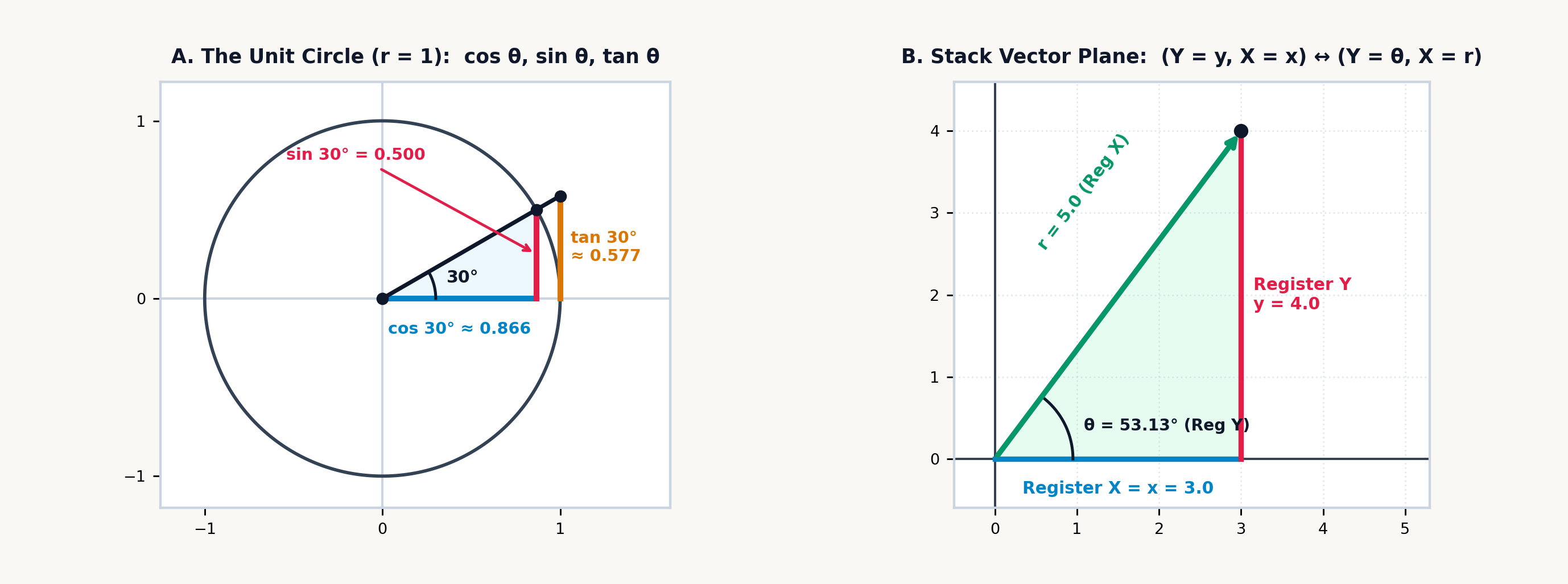
Every triangulation chain rests on a single geometric principle: translating a sighted angle into a ratio of straight-line distances by inscribing a right triangle inside a circle of unit radius. When a circle of radius \(r = 1\) is centered at the origin of an \((x, y)\) coordinate plane—the Unit Circle—and a radial vector is rotated counterclockwise from the positive horizontal axis through an angle \(\theta\), the tip of that vector defines a right triangle of hypotenuse \(1\) (Figure 4.1):
Physical CPA Studio Bridge (
Book 4 Units 05–06— Unit Circle Volvelle & 84.0 mm Comparator):
In the companion StackCalc High School & STEM Lab (Book 4, Units 05–06), students pair the two-disc rotating \(120\text{ mm}\) Unit Circle & Trig Volvelle with the \(84.0\text{ mm}\) Fraction Comparator to measure \((\cos\theta, \sin\theta)\) horizontal and vertical projections physically before evaluating trigonometric functions and polar–rectangular coordinate projections on the \((Y, X)\) stack. Dialing the Volvelle pointer to \(\theta = 30^\circ\) aligns the vertical sine sight-window with the \(\frac{1}{2}\) fraction block (\(42.0\text{ mm}\) out of \(84.0\text{ mm}\), \(\sin 30^\circ = 0.5\)), turning abstract phasor decompositions into direct caliper and comparator measurements.
As the unit radius arm (\(r = 1\)) rotates counterclockwise from \(0^\circ\) to \(30^\circ\) (\(\pi/6\text{ rad}\)), it frames the right-triangle projections on the horizontal and vertical axes:
As the radius vector rotates past \(45^\circ\), where \(\cos 45^\circ = \sin 45^\circ = \sqrt{2}/2 \approx 0.707\), and \(60^\circ\), where \(\cos 60^\circ = 1/2\) and \(\sin 60^\circ = \sqrt{3}/2\), it reaches the vertical axis at \(90^\circ\), where the horizontal projection vanishes to \(\cos 90^\circ = 0\) and the vertical projection reaches \(\sin 90^\circ = 1\). The third circular ratio, the tangent \(\tan\theta = \sin\theta / \cos\theta\), measures the vertical height where the extended radius ray intersects the tangent line \(x = 1\) at the right edge of the unit circle.
4.1.1 Three Ways to Slice a Circle: Degrees, Radians, and Gradians
Before evaluating a trigonometric function, the angular unit that subdivides a full revolution around the unit circle must be selected across the three standard engineering conventions:
| Angular Mode | Full Circle Revolution | Right Angle | Primary Engineering Field |
|---|---|---|---|
| Degrees | \(360^\circ\) | \(90^\circ\) | Structural Civil Engineering, Geodesy, Avionics |
| Radians | \(2\pi \approx 6.283\text{ rad}\) | \(\pi/2 \approx 1.571\text{ rad}\) | Mathematical Physics, Calculus, Wave Mechanics |
| Gradians | \(400\text{ grad}\) | \(100\text{ grad}\) | European Surveying, Mining Engineering |
All three conventions remain in engineering use because each serves a distinct structural symmetry. In sexagesimal (base-\(60\)) arithmetic, \(360\) is a highly composite integer divisible without remainder by \(2, 3, 4, 5, 6, 8, 9, 10, 12, 15, 18, 20, 24, 30, 36, 40, 45, 60, 72, 90, 120,\) and \(180\), so degrees allow a machinist, surveyor, or navigator to subdivide a circle into halves, thirds, quarters, fifths, sixths, eighths, or twelfths using exact integers.
In mathematical analysis, dividing a circle into \(360\) parts is an external convention. Radian measure defines the unit angle \(\theta\) intrinsically from the circle itself as the central angle subtending an arc whose length \(s\) equals the radius \(r\). Defining an angle as the dimensionless ratio of arc length to radius (\(\theta = s / r\)) makes one full revolution equal to \(2\pi\text{ radians}\) (\(\approx 6.283\text{ rad}\)) and one radian equal to \(180^\circ / \pi \approx 57.296^\circ\). Only in radians does the small-angle limit \(\lim_{\theta \to 0} (\sin\theta)/\theta\) equal \(1\), so that \(\frac{d}{d\theta}\sin\theta = \cos\theta\) without introducing a factor of \(\pi/180\) into differential equations of harmonic oscillation or wave propagation.
Gradians decimalize angular measure by defining a right angle as \(100\text{ gradians}\) (gons) and a full circle as \(400\text{ gradians}\). Because the metric quadrant from the Equator to the North Pole spans \(10,000\text{ km}\) per \(100\text{ grad}\), one gradian of latitude corresponds to \(100\text{ kilometers}\) along a meridian, one centigrad (\(0.01\text{ grad}\), or one decimal arcminute) corresponds to \(1\text{ kilometer}\), and \(10^{-5}\text{ grad}\) corresponds to \(1\text{ meter}\).
When a nautical chart or surveyor's plat specifies an angle in sexagesimal degrees, arcminutes, and arcseconds (\(D^\circ M' S''\), packed as D.MMSS, so \(35^\circ 15' 36''\) enters as 35.1536), converting to decimal degrees evaluates the base-\(60\) expansion \(D + M/60 + S/3600 = 35 + 15/60 + 36/3600 = 35.26^\circ\), which in turn scales by \(\pi/180^\circ\) to \(\approx 0.615\text{ radians}\). Before starting a trigonometric calculation, a quick check on \(\sin(45)\) confirms the active angular convention: in radians, \(\sin(45\text{ rad}) \approx 0.851\), while in degrees, \(\sin(45^\circ) = \sqrt{2}/2 \approx 0.707\) and \(\cos(60^\circ) = 0.5\).
A generic floating-point environment evaluating \(\cos(90^\circ)\) frequently returns a non-zero residual of \(6.12 \times 10^{-17}\) instead of exact zero. Inside a conventional math library, an angle in degrees is first converted to radians by multiplying by \(\pi / 180\), so \(90^\circ\) becomes a floating-point approximation to \(\pi / 2\). Because \(\pi\) is transcendental, its binary expansion does not terminate; an IEEE-754 double-precision register truncates \(\pi/2\) after 53 significand bits, producing a value that differs from mathematical \(\pi/2\) by approximately \(6.12 \times 10^{-17}\text{ radians}\).
Near \(\theta = \pi/2\), the derivative of \(\cos\theta\) is \(-\sin(\pi/2) = -1\), so evaluating the cosine polynomial on that truncated binary approximation leaves a \(6.12 \times 10^{-17}\) residual. In a structural stiffness matrix or coordinate transformation, a spurious non-zero entry of \(6.12 \times 10^{-17}\) can propagate into subsequent divisions or prevent zero-threshold tests from matching.
To prevent binary radian conversion from perturbing orthogonal geometry, the SC-32 performs exact axial angle clamping prior to polynomial evaluation: in degree or gradian measure, integer multiples of \(45^\circ\) and \(90^\circ\) are reduced modulo a full circle so that \(\sin(0^\circ) = 0\), \(\cos(0^\circ) = 1\), \(\sin(90^\circ) = 1\), \(\cos(90^\circ) = 0\), \(\sin(180^\circ) = 0\), \(\cos(180^\circ) = -1\), \(\sin(270^\circ) = -1\), \(\cos(270^\circ) = 0\), and \(\tan(\pm 45^\circ) = \pm 1\) return exact IEEE-754 zero and unity values. Evaluating \(\tan(90^\circ)\) or \(\tan(270^\circ)\) traps the vertical asymptote without returning a spurious \(1.63 \times 10^{16}\) reciprocal of rounding noise, and passing an argument \(|x| > 1\) to \(\arcsin x\) or \(\arccos x\) halts without altering the operational stack.
For non-axial angles, the SC-32 evaluates \(\sin x\), \(\cos x\), and \(\tan x\) via octant range reduction: any radian angle \(x\) is decomposed into its nearest integer multiple \(k = \lfloor \frac{2}{\pi}x + \frac{1}{2}\rfloor\) of \(\pi/2\) and a reduced argument \(r = (x - k C_1) - k C_2 \in [-\pi/4, +\pi/4]\), where \(\pi/2 = C_1 + C_2\) is split into an exact high-precision floating-point constant \(C_1\) and an extended-precision residual \(C_2\) so subtracting \(k(\pi/2)\) never suffers catastrophic cancellation. Inside \(|r| \le \pi/4 \approx 0.785\), the alternating Taylor–Maclaurin series converges rapidly:
At \(\theta = 30^\circ\), converting to radians yields \(r = \pi/6 \approx 0.524\text{ rad}\): summing just the first two terms \(r - r^3/6\) already comes within \(0.065\%\) of the exact half-chord, and adding the fifth-power term \(+r^5/120\) reproduces \(\sin(30^\circ) = 0.5\) to within \(2.1 \times 10^{-6}\).
4.1.2 Cannonballs, Inclined Planes, and Unclimbed Peaks
Across classical mechanics and civil surveying, planar trigonometric projections resolve a directed magnitude into orthogonal components along horizontal and vertical axes. Because every circular function (SIN, COS, TAN) is a unary operation that replaces an angle with its dimensionless unit-circle projection, any baseline distance or velocity waiting on the stack can be scaled without intermediate storage.
The parabolic trajectory of a projectile in a uniform gravitational field (neglecting air resistance) is the superposition of two independent orthogonal motions (Galilei, 1638). Horizontally, no net force acts after launch, so the horizontal velocity component \(v_{0x} = v_0\cos\theta\) remains constant downrange. Vertically, gravity \(g\) produces a constant downward acceleration that decelerates the initial vertical component \(v_{0y} = v_0\sin\theta\) until the projectile reaches its apex altitude \(H_{\max}\), where the vertical kinetic energy \(\frac{1}{2}mv_{0y}^2\) equals the gravitational potential energy \(mgH_{\max}\):
By the double-angle identity \(2\sin\theta\cos\theta = \sin(2\theta)\), maximum horizontal range over level ground occurs when \(\sin(2\theta) = 1\) (\(\theta = 45^\circ\)), and any two complementary launch angles summing to \(90^\circ\) (such as \(30^\circ\) and \(60^\circ\)) produce the same downrange distance \(R\). For an artillery shell leaving the muzzle at \(v_0 = 85\text{ m/s}\) inclined at \(\theta = 38^\circ\) (\(g \approx 9.807\text{ m/s}^2\)), the vertical launch velocity \(v_{0y} = 85\sin(38^\circ) \approx 52.331\text{ m/s}\) carries the shell to an apex altitude of \(H_{\max} = v_{0y}^2 / (2g) \approx \mathbf{139.628\text{ m}}\), while scaling the double-angle factor \(\sin(2\theta) = \sin(76^\circ) \approx 0.97\) by \(v_0^2 / g\) resolves the horizontal downrange distance \(R \approx \mathbf{714.86\text{ m}}\).
The same orthogonal resolution governs a mass \(m\) sliding down a plane inclined at angle \(\theta\) with kinetic friction coefficient \(\mu_k\). Gravity acts vertically downward with magnitude \(mg\), while the surface constrains motion along the incline. Resolving the gravitational vector into components parallel and normal to the surface shows that \(mg\sin\theta\) acts down the slope while \(mg\cos\theta\) acts perpendicular to the surface, producing a normal reaction \(N = mg\cos\theta\) and an opposing friction force \(\mu_k N = \mu_k mg\cos\theta\):
Because the mass \(m\) cancels out of both terms, bodies of any mass sharing the same coefficient \(\mu_k\) accelerate down the incline at the same rate, and at the critical angle of repose where \(\sin\theta = \mu_k\cos\theta\) (\(\tan\theta = \mu_k\)), the downslope gravitational component and upslope friction balance to zero. Along a ramp tilted at \(\theta = 34^\circ\) with \(\mu_k = 0.22\) (\(g \approx 9.807\text{ m/s}^2\)), subtracting \(0.22\cos(34^\circ) \approx 0.182\) from \(\sin(34^\circ) \approx 0.559\) gives the net traction factor \(\approx 0.377\), and multiplying by \(g\) yields \(a \approx \mathbf{3.695\text{ m/s}^2}\).
When an inaccessible summit cannot be plumbed by a vertical drop line, two-station optical leveling determines its elevation from a surveyed horizontal baseline: sighting the vertical elevation angle \(\alpha\) to the summit from Station 1, advancing a measured horizontal baseline distance \(d\) toward the peak to Station 2, and sighting the steeper elevation angle \(\beta\). Because the horizontal distances from the summit's plumb line to the two stations are \(x_1 = H\cot\alpha\) and \(x_2 = H\cot\beta\), their difference \(x_1 - x_2 = d\) eliminates the unmeasured horizontal distance to the mountain's interior plumb line:
Since \(\sec\theta = 1/\cos\theta\), \(\csc\theta = 1/\sin\theta\), and \(\cot\theta = 1/\tan\theta\) are the multiplicative reciprocals of the three primary circular ratios, dedicated keys for secant, cosecant, and cotangent are unnecessary: across a level baseline of \(d = 500\text{ m}\) with elevation angles \(\alpha = 24.5^\circ\) at Station 1 and \(\beta = 31.2^\circ\) at Station 2, the cotangent difference \(\cot(24.5^\circ) - \cot(31.2^\circ) \approx 0.543\text{ m/m}\) yields the summit height \(H \approx \mathbf{920.635\text{ meters}}\).
When the horizontal baseline \(D\) to the base of a vertical target is known—as in forestry timber cruising with a handheld optical clinometer—readings of the inclination angle \(\theta_{\text{top}} = +52^\circ\) to a Douglas fir's crown leader and the depression angle \(\theta_{\text{base}} = -8^\circ\) to its root collar at \(D = 30\text{ m}\) give total tree height \(H = D(\tan\theta_{\text{top}} - \tan\theta_{\text{base}}) \approx 30(1.42) \approx \mathbf{42.614\text{ m}}\). In a precision toolroom machine shop, setting up a surface grinder with a hardened steel sine bar of center-to-center roller spacing \(L = 5\text{ in}\) uses the vertical sine projection \(h = L\sin\theta = 5\sin(14^\circ 15') \approx \mathbf{1.231\text{ in}}\) (wrung from \(0.101'' + 0.13'' + 1''\) gauge blocks) to establish a taper angle of \(\theta = 14^\circ 15' 00''\).
Circular projection also governs the period of a simple pendulum: at finite angular amplitude \(\theta_0\), the exact gravitational restoring torque \(\sin\theta\) is smaller than the linearized approximation \(\theta\), lengthening the small-angle period \(T_0 = 2\pi\sqrt{L/g}\) according to the leading half-angle sine term \(T \approx T_0[1 + \frac{1}{4}\sin^2(\theta_0/2)]\). For a clock pendulum (\(T_0 = 2\text{ s}\)) released from \(\theta_0 = 45^\circ\), this finite-amplitude correction yields \(T \approx \mathbf{2.073\text{ seconds}}\) (\(+3.66\%\)).
4.1.3 Bending Light and Diffracting X-Rays
Whereas forward trigonometric functions map an angle to a dimensionless ratio of lengths, inverse trigonometric functions (ASIN, ACOS, ATAN) reverse that mapping, recovering the geometric angle from a measured ratio of phase velocities, refractive indices, wavelengths, or accelerations. Across geometric and physical optics, every boundary condition and interference fringe stems from a single wave principle: when a wavefront crosses an interface or passes through an aperture, phase continuity along the boundary ties the sine or cosine of the propagation angle to the ratio of wavelengths or phase speeds.
Across a boundary between two optical media of refractive indices \(n_1\) and \(n_2\) (where light travels at phase velocities \(v_1 = c/n_1\) and \(v_2 = c/n_2\)), a ray arriving at incidence angle \(\theta_1\) to the surface normal bends to a refracted angle \(\theta_2\) so that the wavefront crests stay phase-locked along the interface. That single phase-matching rule—Snell's law of refraction—also governs three limiting angles of optical engineering: the critical angle \(\theta_c\) for total internal reflection inside a high-index core (\(n_1 > n_2\)), the Numerical Aperture \(\text{NA}\) measuring the light-gathering half-cone \(\theta_{\max}\) of an optical fiber in an external medium of index \(n_0\), and Brewster's polarization angle \(\theta_B\), where reflected and refracted rays meet at right angles:
Steepening the incidence angle inside a denser core (\(n_1 > n_2\)) bends the refracted ray closer and closer to the interface until it skims along the boundary at \(\theta_2 = 90^\circ\) (\(\sin 90^\circ = 1\)); solving \(n_1\sin\theta_c = n_2\) gives \(\theta_c = \arcsin(n_2/n_1)\), beyond which \(100\%\) of the wave reflects internally. Applying the Pythagorean identity \(\cos^2\theta_c = 1 - (n_2/n_1)^2\) at that grazing limit defines the fiber's numerical aperture \(\text{NA} = \sqrt{n_1^2 - n_2^2} = n_0\sin\theta_{\max}\), fixing the widest external cone \(\theta_{\max}\) that can enter the core and stay guided. When the reflected ray (at angle \(\theta_B\)) and refracted ray (at angle \(\theta_2\)) meet at right angles (\(\theta_B + \theta_2 = 90^\circ\)), \(\sin\theta_2 = \cos\theta_B\) and Snell's law \(n_1\sin\theta_B = n_2\cos\theta_B\) reduces to \(\tan\theta_B = n_2/n_1\).
For a ray entering crown glass (\(n_2 = 1.52\)) from air (\(n_1 = 1.0003\)) at incidence angle \(\theta_1 = 40^\circ\), \(\arcsin(1.0003\sin 40^\circ / 1.52)\) yields the refracted angle \(\theta_2 \approx \mathbf{25.025^\circ}\). When laser light propagates from a denser silica optical fiber core (\(n_1 = 1.48\)) toward a lower-index cladding (\(n_2 = 1.45\)), dividing \(n_2 / n_1 \approx 0.98\) and taking the arcsine determines the critical total-internal-reflection angle \(\theta_c \approx \mathbf{78.444^\circ}\), while the fiber's Numerical Aperture \(\text{NA} = \sqrt{n_1^2 - n_2^2} \approx \mathbf{0.296}\) sets the maximum external acceptance half-cone \(\theta_{\max} = \arcsin(\text{NA}) \approx \mathbf{17.246^\circ}\) in air (\(n_0 = 1\)).
At the same dielectric interface, the fraction of wave energy reflected versus transmitted depends on the polarization of the electric-field vector relative to the boundary plane. At normal incidence across an uncoated air-to-crown-glass lens surface (\(n_1 = 1, n_2 = 1.52\)), Fresnel reflection returns \(R_{\perp} = \left(\frac{n_1 - n_2}{n_1 + n_2}\right)^2 = \left(\frac{-0.52}{2.52}\right)^2 \approx \mathbf{4.258\%}\) of incident light per surface. At oblique incidence at Brewster's angle \(\theta_B = \arctan(n_2/n_1)\), oscillating dipoles in the glass cannot radiate transverse waves along their own oscillation axis, so reflected light becomes completely linearly polarized parallel to the surface (for air to flint glass with \(n_1 = 1, n_2 = 1.62\), \(\arctan(1.62) \approx \mathbf{58.314^\circ}\)).
Once light is linearly polarized with irradiance \(I_0 = 80\text{ W/m}^2\) and passes through a second analyzer rotated by \(\theta = 35^\circ\), Malus's law projects the electric-field vector as \(E_0\cos\theta\), scaling transmitted intensity by the squared cosine \(I(\theta) = I_0\cos^2(35^\circ) \approx \mathbf{53.681\text{ W/m}^2}\). The same orthogonal force-ratio geometry (\(\tan\theta = F_x / F_y\)) that sets Brewster's angle in optics also resolves the zero-slip banking angle of a highway curve of radius \(R = 350\text{ m}\) at \(v = 100\text{ km/h}\) (\(\approx 27.778\text{ m/s}\), \(g \approx 9.807\text{ m/s}^2\)): equating horizontal centripetal acceleration \(v^2/R\) with the horizontal projection of normal force gives \(\theta_{\text{bank}} = \arctan(v^2 / gR) \approx \mathbf{12.67^\circ}\).
When coherent wavefronts of wavelength \(\lambda\) pass through an optical diffraction grating of slit spacing \(d\) (deflected at angle \(\theta_m\) for integer diffraction order \(m\)) or reflect at grazing Bragg angle \(\theta_B\) from parallel atomic crystal planes separated by interplanar lattice spacing \(d\) (at integer reflection order \(n\)), constructive interference occurs wherever neighboring rays arrive in phase by a whole number of wavelengths; similarly, when a star's light ray arriving at rest-frame angle \(\theta\) is observed from a spacecraft moving at relativistic speed fraction \(\beta = v/c\), Lorentz transformation of the wavefront normal shifts the apparent viewing angle to \(\theta'\):
Waves emerging from adjacent slits of a transmission grating accumulate the slant path difference \(d\sin\theta_m\) only once, whereas an X-ray wave penetrating to a deeper crystal plane traverses that slant step \(d\sin\theta_B\) twice—once descending to the lower atomic sheet and once reflecting back out—introducing the factor of \(2\) in \(2d\sin\theta_B = n\lambda\). For the relativistic observer, Lorentz contraction and time dilation combine in \((\cos\theta - \beta)/(1 - \beta\cos\theta)\) to sweep incoming starlight forward into a narrow searchlight cone ahead of the spacecraft.
In an optical diffraction grating, monochromatic green light of wavelength \(\lambda = 532\text{ nm}\) (\(5.32 \times 10^{-7}\text{ m}\)) illuminating a grating ruled at \(N = 600\text{ lines/mm}\) (slit pitch \(d = 1 / 600,000\text{ m} \approx 1.667\,\mu\text{m}\)) produces its second-order principal maximum (\(m = 2\)) at \(\theta_2 = \arcsin(2\lambda / d) \approx \mathbf{39.673^\circ}\). At atomic length scales, Bragg X-ray diffraction of wavelength \(\lambda \approx 0.154\text{ nm}\) (\(\text{Cu K}\alpha\)) reflected from parallel silicon \((111)\) lattice planes at glancing angle \(\theta_B = 14.22^\circ\) (\(n = 1\)) reveals an interplanar spacing of \(d = \lambda / (2\sin 14.22^\circ) \approx \mathbf{0.313\text{ nm}}\). And when a distant star's light arrives at \(\theta = 60^\circ\) (\(\cos\theta = 0.5\)) in the rest frame of a spacecraft moving at \(\beta = v/c = 0.5\), relativistic aberration shifts the ray's apparent direction to the transverse angle \(\cos\theta' = 0 \implies \theta' = \mathbf{90^\circ}\) (because the incoming ray's longitudinal velocity projection \(c\cos 60^\circ = 0.5c\) matches the spacecraft's forward speed \(v = 0.5c\)).
4.2 Triangles Across Land, Sea, and Air
Geodetic surveying, structural truss analysis, and wave interference rarely involve right-angled triangles. When a surveyor occupies a corner station \(C\) and measures straight-line distances \(a\) and \(b\) to two boundary monuments separated by an included angle \(C \ne 90^\circ\), dropping an altitude \(h\) from the vertex opposite side \(a\) decomposes the oblique triangle into two right triangles. In the inner right triangle containing angle \(C\), the vertical altitude has length \(h = b\sin C\), while the horizontal projection of side \(b\) along side \(a\) has length \(b\cos C\), so the remaining base of the outer right triangle is \((a - b\cos C)\). Applying the Pythagorean theorem to that outer right triangle and simplifying via \(\cos^2 C + \sin^2 C = 1\) yields the Law of Cosines:
Subtracting the projection cross-term \(2ab\cos C\) generalizes the Pythagorean sum \(a^2 + b^2\) to any planar triangle. When \(C = 90^\circ\), \(\cos 90^\circ = 0\) and the cross-term vanishes, recovering the Pythagorean theorem (\(c = \sqrt{a^2 + b^2}\)); when \(C < 90^\circ\) (an acute angle), \(\cos C > 0\) draws the opposite side \(c\) shorter than the right-triangle hypotenuse; and when \(C > 90^\circ\) (an obtuse angle), \(\cos C < 0\) makes \(-2ab\cos C\) positive and stretches \(c\) longer. Replacing the interior angle \(C\) with the exterior supplement \(180^\circ - \Delta\phi\) reverses the sign of the cosine term and yields the law of coherent wave interference for two acoustic or electromagnetic phasors of amplitudes \(A_1\) and \(A_2\) arriving with phase difference \(\Delta\phi\):
For a boundary corner with sides \(a = 45\text{ m}\) and \(b = 62\text{ m}\) separated by \(C = 48^\circ\), subtracting \(2(45)(62)\cos 48^\circ \approx 3,733.749\text{ m}^2\) from the Pythagorean sum \(a^2 + b^2 = 5,869\text{ m}^2\) and taking the square root yields the opposite boundary side \(c \approx \mathbf{46.209\text{ m}}\); for two coherent sound waves of amplitudes \(A_1 = 2.4\text{ Pa}\) and \(A_2 = 3.1\text{ Pa}\) interfering at phase angle \(\Delta\phi = 55^\circ\), adding \(2(2.4)(3.1)\cos 55^\circ \approx 8.535\text{ Pa}^2\) to \(A_1^2 + A_2^2 = 15.37\text{ Pa}^2\) and taking the square root resolves the resultant amplitude \(A_{\text{res}} \approx \mathbf{4.889\text{ Pa}}\).
When the Law of Cosines is applied across two supplementary sub-triangles that share a common line, the opposing cosines cancel (\(\cos\theta + \cos(180^\circ - \theta) = 0\)) and produce three purely algebraic distance and area laws without angles. First, in a triangle of outer sides \((a, b, c)\) where an internal tie-rod (cevian) of length \(d\) divides base \(a\) into segments \(m\) and \(n\) (\(m + n = a\)), canceling the supplementary cosines at the base yields Stewart's cevian theorem. Second and third, when a four-sided polygon of side lengths \((a, b, c, d)\), semiperimeter \(s = \frac{1}{2}(a + b + c + d)\), and interior diagonals \(p\) and \(q\) is inscribed inside a circle (a cyclic quadrilateral), its opposite vertex angles sum to \(180^\circ\); canceling their equal-and-opposite cosines yields Brahmagupta's area formula for the enclosed area \(K\) and Ptolemy's theorem relating the diagonals \(p, q\) to the four sides:
Stewart's relation weights the squared outer sides by their opposite base segments—\((b^2 m + c^2 n)/a\)—and subtracts the segment product \(mn\) to isolate the squared internal strut \(d^2\) directly from linear lengths. Brahmagupta's radical \(K = \sqrt{(s-a)(s-b)(s-c)(s-d)}\) treats all four sides symmetrically around the semiperimeter \(s\), reducing to Heron's triangle formula \(\sqrt{s(s-a)(s-b)(s-c)}\) whenever the fourth side \(d\) shrinks to zero, while Ptolemy's identity \(p \cdot q = ac + bd\) equates the product of the two interior diagonals to the sum of the opposite-side products.
For a roof truss triangle with sides \(b = 13\text{ m}\), \(c = 15\text{ m}\), and base \(a = 14\text{ m}\) split into segments \(m = 6\text{ m}\) (adjacent to side \(c\)) and \(n = 8\text{ m}\) (adjacent to side \(b\)), Stewart's theorem determines the internal tie-rod length \(d = \sqrt{201 - 48} \approx \mathbf{12.369\text{ m}}\) from the side lengths alone; for a cyclic quadrilateral with sides \(a = 5, b = 6, c = 7, d = 8\) (semiperimeter \(s = 13\)), Brahmagupta's radical gives area \(K = \sqrt{8 \times 7 \times 6 \times 5} \approx \mathbf{40.988}\) while Ptolemy's opposite-side sum gives the diagonal product \(pq = 5(7) + 6(8) = \mathbf{83}\).
The altitude \(h = b\sin C = c\sin B\) dropped to base \(a\) establishes the Law of Sines, the circumcircle diameter \(2R_{\text{circ}}\), and the two-side included-angle cross-product area \(K = \frac{1}{2}ab\sin C\) (paired with the semiperimeter \(s = \frac{1}{2}(a + b + c)\) and the inscribed circle radius \(r_{\text{in}} = K/s\)):
For the roof truss triangle with sides \(a = 14\text{ m}, b = 13\text{ m}, c = 15\text{ m}\) (\(s = 21\text{ m}\)) and enclosed area \(K = \mathbf{84\text{ m}^2}\), these relations determine the included vertex angle \(C = \arcsin\!\left(\frac{2K}{ab}\right) \approx \mathbf{67.38^\circ}\), the circumcircle radius \(R_{\text{circ}} = \frac{abc}{4K} = \mathbf{8.125\text{ m}}\), and the incircle radius \(r_{\text{in}} = K/s = \mathbf{4\text{ m}}\).
4.2.1 The Two-Register Vector Plane
In scalar arithmetic, binary operators treat Registers \(Y\) and \(X\) as two scalar operands that collapse into a single result. In two-dimensional vector geometry, Registers \(Y\) and \(X\) operate together as a coordinate pair representing a point or vector in the plane. Navigators, surveyors, and electrical engineers convert continuously between polar coordinates \((r, \theta)\) and rectangular coordinates \((x, y)\) because field instruments measure in polar form while vector addition requires rectangular components. When a radar antenna tracks a target, a surveyor sights a monument with a theodolite, or an aircraft instrument panel displays airspeed and heading, the measurement consists of a radial magnitude \(r\) and a direction angle \(\theta\).
By the parallelogram law of forces, non-collinear vectors cannot be summed by adding their scalar magnitudes \(r_1 + r_2\). To combine an aircraft's airspeed vector with a crosswind, or to verify that a multi-leg property survey closes back onto its starting monument, each polar vector \((r, \theta)\) must first be resolved into its horizontal component (\(x = r\cos\theta\)) and vertical component (\(y = r\sin\theta\)), summed along each orthogonal axis (\(\Sigma x, \Sigma y\)), and converted back into a resultant magnitude \(r\) and direction \(\theta\).
With the primary horizontal coordinate \(x\) and radial magnitude \(r\) in Register \(X\) (Line 1) and the vertical coordinate \(y\) and direction angle \(\theta\) in Register \(Y\) (Line 2), both components remain visible together: rectangular-to-polar conversion maps \((Y = y,\; X = x)\) in place to \((Y = \theta = \operatorname{atan2}(y, x),\; X = r = \sqrt{x^2 + y^2})\), and polar-to-rectangular projection maps \((Y = \theta,\; X = r)\) in place to \((Y = y = r\sin\theta,\; X = x = r\cos\theta)\) without disturbing Registers \(Z\) or \(T\).
The two-argument rectangular-to-polar transformation avoids the quadrant ambiguity and axial singularity of dividing \(y / x\) and taking a scalar \(\arctan(y/x)\), which receives only the single scalar quotient \(y/x\). In Quadrant III, where both \(x = -3\) and \(y = -4\) are negative, the quotient \((-4)/(-3) \approx +1.333\) is positive, so \(\arctan(y/x)\) returns \(\approx +53.13^\circ\) in Quadrant I, an error of \(180^\circ\); on the positive or negative vertical axis where \(x = 0\) and \(y = \pm 10\), dividing \(y/x\) encounters a division-by-zero singularity. The four-quadrant \(\operatorname{atan2}(y, x)\) function resolves this ambiguity by inspecting the individual signs of \(y\) in Register \(Y\) and \(x\) in Register \(X\) across the full \((-180^\circ, +180^\circ]\) circle:
| Quadrant / Axis | Signs of \((x, y)\) | Four-Quadrant \(\operatorname{atan2}(y, x)\) Formula (in DEG) |
Example Vector \((x, y)\) | Output \((Y = \theta, X = r)\) |
|---|---|---|---|---|
| Quadrant I | \(x > 0,\; y \ge 0\) | \(\arctan(y/x)\) | \((+3, +4)\) | \(\theta \approx +53.13^\circ,\; r = 5\) |
| Quadrant II | \(x < 0,\; y \ge 0\) | \(\arctan(y/x) + 180^\circ\) | \((-3, +4)\) | \(\theta \approx +126.87^\circ,\; r = 5\) |
| Quadrant III | \(x < 0,\; y < 0\) | \(\arctan(y/x) - 180^\circ\) | \((-3, -4)\) | \(\theta \approx -126.87^\circ,\; r = 5\) |
| Quadrant IV | \(x > 0,\; y < 0\) | \(\arctan(y/x)\) | \((+3, -4)\) | \(\theta \approx -53.13^\circ,\; r = 5\) |
| Vertical Axes | \(x = 0,\; y \ne 0\) | \(+90^\circ\) if \(y > 0\), \(-90^\circ\) if \(y < 0\) | \((0, +10)\) | \(\theta = +90^\circ,\; r = 10\) |
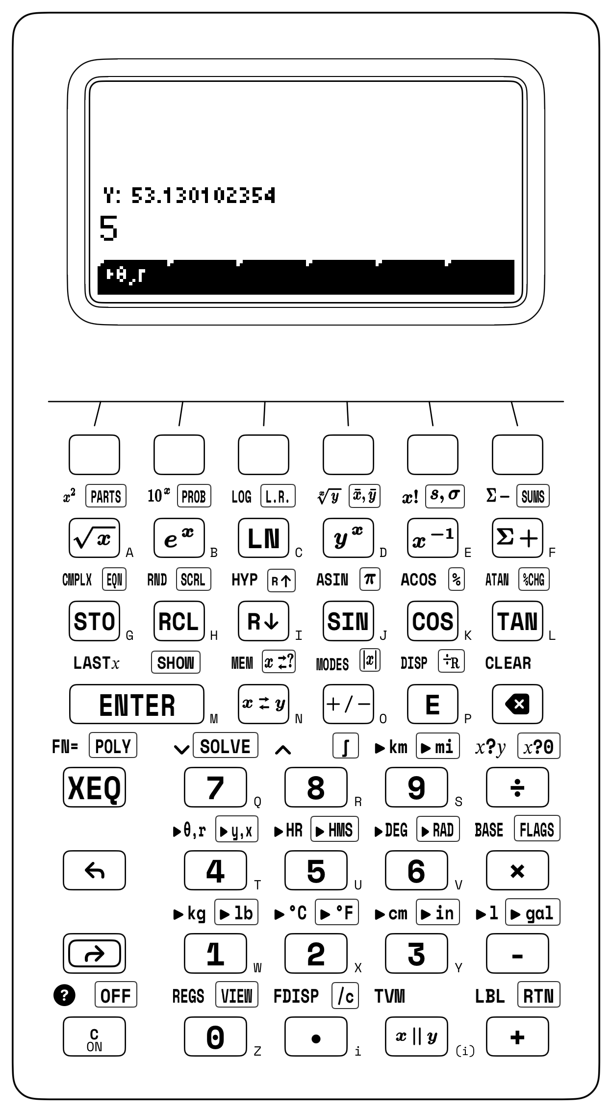
A vector of radius \(r = 10\) along the positive vertical axis (\(\theta = 90^\circ\)) illustrates the register mapping: placing angle \(\theta\) in Register \(Y\) and radius \(r\) in Register \(X\) yields \(0\) in Register \(X\) (\(x = 10\cos 90^\circ\)) and \(10\) in Register \(Y\) (\(y = 10\sin 90^\circ\)). In the inverse direction, converting a \(3\text{-}4\text{-}5\) right triangle (\(y = 4\) in Register \(Y\), \(x = 3\) in Register \(X\)) places the angle \(\theta \approx 53.13^\circ\) in Register \(Y\) and the hypotenuse \(r = 5\) in Register \(X\).
When a land surveyor or navigator records the distance \(r_i\) and North Azimuth \(\alpha_i\) (measured clockwise from True North, where \(0^\circ = \text{North}\) and \(90^\circ = \text{East}\)) around a closed property boundary, reflecting the coordinate axes across the \(45^\circ\) Northeast diagonal swaps sine and cosine so that Northing latitude is \(\Delta N_i = r_i\cos\alpha_i\) and Easting departure is \(\Delta E_i = r_i\sin\alpha_i\):
Because polar-to-rectangular projection evaluates \((Y = r\sin\theta,\; X = r\cos\theta)\), entering a Cartesian angle \(\theta\) (counterclockwise from East) produces \((Y = \Delta y,\; X = \Delta x)\), while entering a surveyor's or pilot's North Azimuth \(\alpha\) (clockwise from North) places Easting departure (\(\Delta E = r\sin\alpha\)) in Register \(Y\) and Northing latitude (\(\Delta N = r\cos\alpha\)) in Register \(X\)—and rectangular-to-polar conversion evaluates \(\operatorname{atan2}(\Delta E, \Delta N)\) to recover the North Azimuth.
Across electrical power engineering and structural mechanics, orthogonal projections resolve directed quantities into active and quadrature components across Registers \(X\) and \(Y\). When an inductive AC motor draws \(I_{\text{rms}} = 8.5\text{ A}\) from a \(V_{\text{rms}} = 120\text{ V}\) line at a lagging phase angle of \(\phi = 32^\circ\), projecting the apparent power \(S = V_{\text{rms}}I_{\text{rms}} = 1,020\text{ VA}\) at \(32^\circ\) resolves real shaft power \(P = S\cos\phi \approx \mathbf{865.01\text{ W}}\) in Register \(X\) and reactive magnetic power \(Q = S\sin\phi \approx \mathbf{540.518\text{ VAR}}\) in Register \(Y\). Even in three-dimensional space frames, the interior mitre angle \(\theta\) between skew struts \(\vec{A} = (4, 6, 8\text{ m})\) (\(|\vec{A}|^2 = 116\text{ m}^2\)) and \(\vec{B} = (2, -3, 5\text{ m})\) (\(|\vec{B}|^2 = 38\text{ m}^2\)) with dot product \(\vec{A}\cdot\vec{B} = 4(2) + 6(-3) + 8(5) = 30\text{ m}^2\) follows from the Cauchy–Schwarz identity \(\cos\theta = \frac{\vec{A}\cdot\vec{B}}{|\vec{A}||\vec{B}|} \approx 0.452\), giving \(\theta \approx \mathbf{63.137^\circ}\).
4.2.2 Great Circles, Migrating Godwits, and the Oblate Earth
Over intercontinental distances, planar Cartesian trigonometry must be replaced by spherical geometry. On a spherical Earth of mean radius \(R_E = 6,371\text{ km}\), the shortest path between two points at latitude/longitude coordinates \((\phi_1, \lambda_1)\) and \((\phi_2, \lambda_2)\) is not a constant-bearing rhumb line (loxodrome) on a Mercator projection, but a great-circle orthodrome: the arc formed on the surface by a plane passing through both points and the center of the Earth.
The Spherical Law of Cosines follows from three-dimensional unit-sphere coordinates. On a sphere of unit radius \(r = 1\), a point at latitude \(\phi\) and longitude \(\lambda\) has polar coordinate \(z = \sin\phi\) and equatorial radius \(\cos\phi\), which projects onto the equatorial \((x, y)\) axes as \(x = \cos\phi\cos\lambda\) and \(y = \cos\phi\sin\lambda\):
Between those two unit vectors, the Euclidean inner product \(\hat{u}_1 \cdot \hat{u}_2 = \cos d\) and the cosine difference identity \(\cos\lambda_1\cos\lambda_2 + \sin\lambda_1\sin\lambda_2 = \cos(\lambda_2 - \lambda_1)\) express the central geocentric angle \(d\) as the sum of the axial projection (\(\sin\phi_1\sin\phi_2\)) and the equatorial projection (\(\cos\phi_1\cos\phi_2\cos\Delta\lambda\)):
Because meridians converge toward the poles as \(\cos\phi\), the great-circle route between San Francisco (\(\phi_1 \approx 37.619^\circ\text{ N}, \lambda_1 = 122.375^\circ\text{ W} = -122.375^\circ\)) and Tokyo Narita (\(\phi_2 = 35.772^\circ\text{ N}, \lambda_2 \approx 140.393^\circ\text{ E}\), longitude span \(\Delta\lambda \approx 97.232^\circ\)) arcs northward toward the Aleutian Islands near \(50^\circ\text{ N}\), where each degree of longitude spans a shorter arc than at \(36^\circ\text{ N}\). Combining the polar axial projection \(\sin\phi_1\sin\phi_2 \approx 0.357\) with the equatorial projection \(\cos\phi_1\cos\phi_2\cos\Delta\lambda \approx -0.081\) gives \(\cos d \approx 0.276\), whose arccosine resolves a central angle of \(d \approx \mathbf{73.983^\circ}\), or \(\approx \mathbf{8,226.6\text{ km}}\) at \(R_E = 6,371\text{ km}\).
The same Spherical Law of Cosines solves the astronomical triangle connecting the North Celestial Pole, an observer's zenith at latitude \(\phi\), and the sun at seasonal declination \(\delta\) and hour angle \(\omega\) (\(15^\circ\) per hour from local solar noon), determining the solar horizon altitude \(\alpha\) and South-referenced azimuth \(\gamma_s\):
At latitude \(\phi = 32^\circ\text{ N}\), declination \(\delta = 18.5^\circ\), and hour angle \(\omega = 45^\circ\), summing the two spherical projections and taking the arcsine locks a solar concentrator onto \(\alpha \approx \mathbf{47.461^\circ}\). Migratory birds combine these same geometric relationships during transoceanic flight: each autumn, the bar-tailed godwit (Limosa lapponica) departs Alaska's tidal flats and flies \(11,000\text{ kilometers}\) non-stop across the Pacific Ocean to New Zealand over nine days, coupling its internal circadian rhythm with solar elevation and geomagnetic inclination cues to follow a great-circle orthodrome while compensating for crosswind drift.
When two waypoints lie only a few meters or kilometers apart (\(d \to 0^\circ\)), \(\cos d\) approaches \(1\), where subtracting from \(1\) in the Spherical Law of Cosines loses significant digits. To eliminate near-zero cosine cancellation in marine and avionics navigation, the Haversine ("half-versed-sine", \(\operatorname{hav}\theta = \frac{1 - \cos\theta}{2} = \sin^2(\theta/2)\)) replaces cosine differences with squared half-angle sines:
For two harbor channel buoys at latitude \(\phi_1 = 37.8^\circ\text{ N}\) and \(\phi_2 = 37.81^\circ\text{ N}\) (\(\Delta\phi/2 = 0.005^\circ\)) and longitude separation \(\Delta\lambda = 0.015^\circ\) (\(\Delta\lambda/2 = 7.5 \times 10^{-3\circ}\)), the Haversine formula evaluates \(\operatorname{hav} d \approx 7.615 \times 10^{-9} + 1.07 \times 10^{-8} \approx 1.831 \times 10^{-8}\) without subtracting \(\cos d \approx 1\) from \(1\), resolving the surface separation \(D = R_E \cdot 2\arcsin(\sqrt{\operatorname{hav} d}) \approx \mathbf{1,724.269\text{ meters}}\) to millimeter precision.
Where satellite navigation requires sub-meter geodetic accuracy, the spherical model is refined to an oblate spheroid. Because Earth's diurnal rotation causes the equatorial radius to exceed the polar radius by \(21.385\text{ km}\)—a bulge large enough that if a smartphone GPS receiver treated Earth as a perfect sphere, its map pin at mid-latitudes would miss the street by nearly \(20\text{ kilometers}\)—the World Geodetic System 1984 (WGS84) reference ellipsoid (equatorial semi-major axis \(a = 6,378,137\text{ m}\), flattening \(f \approx 1/298.257\), first eccentricity squared \(e^2 = 2f - f^2 \approx 6.694 \times 10^{-3}\)) defines the prime-vertical radius of curvature \(N(\phi)\) and Earth-Centered Earth-Fixed coordinates \((X, Y, Z)\) at geodetic latitude \(\phi\), longitude \(\lambda\), and ellipsoidal height \(h\):
At mid-latitude \(\phi = 45^\circ\text{ N}\) (\(\sin^2 45^\circ = 0.5\)), dividing \(a = 6,378,137\text{ m}\) by \(\sqrt{1 - 0.5 e^2}\) yields a prime-vertical radius of curvature of \(N(45^\circ) \approx \mathbf{6,388,838.29\text{ m}}\).
4.2.3 Hanging Chains, Standing Arches, and the Unit Hyperbola
A flexible chain hanging under its own weight curves into a hyperbolic cosine, not a quadratic parabola, because of how its load is distributed. Whereas a quadratic parabola (\(y = kx^2\)) arises only when vertical load is distributed uniformly per unit of horizontal span \(dx\) (as in a suspension-bridge cable supporting a flat roadway deck), an unburdened hanging chain distributes its weight uniformly per unit of curved arc length \(ds = \sqrt{1 + (dy/dx)^2}\,dx\).
For a chain segment of arc length \(s\) in static equilibrium between the lowest vertex (horizontal tension \(T_0\)) and a point \((x, y)\) at tangent angle \(\psi\), horizontal tension stays constant at \(T\cos\psi = T_0\) while vertical support balances the cable weight \(T\sin\psi = w \cdot s\), where \(w\) is the weight per unit length in \(\text{N/m}\). Dividing the vertical balance by the horizontal balance relates the local slope \(\frac{dy}{dx} = \tan\psi\) to the arc length \(s\):
A derivative with respect to \(x\) gives \(\frac{d^2 y}{dx^2} = \frac{1}{a}\frac{ds}{dx} = \frac{1}{a}\sqrt{1 + (dy/dx)^2}\), whose solution is the symmetric mean of rising and decaying exponentials \(e^{x/a}\) and \(e^{-x/a}\). This curve is the catenary (from the Latin catena, "chain"), governed by the hyperbolic cosine:
With the origin placed at the lowest vertex of the span, the vertical rise \(y(x)\) follows the shifted hyperbolic cosine, the arc length \(s(x)\) measured from the vertex to \(x\) follows the hyperbolic sine, and the local cable tension \(T(x) = \sqrt{T_0^2 + (ws)^2}\) is proportional to the height \(y + a\):
These exponential combinations are termed hyperbolic functions and share keys with \(\sin\), \(\cos\), and \(\tan\) because while the circular functions \((\cos u, \sin u)\) parameterize the unit circle \(x^2 + y^2 = 1\) (sweeping out a circular sector of area \(u/2\)), squaring and subtracting \(\cosh u\) and \(\sinh u\) shows that \((\cosh u, \sinh u)\) parameterize the right branch of the unit hyperbola \(x^2 - y^2 = 1\) (sweeping out a hyperbolic sector of area \(u/2\)):
Their derivatives parallel the circular functions without sign reversal on \(\frac{d}{du}\cosh u\):
When inverted into an arch, a hanging catenary curve exchanges pure axial tension for pure axial compression without bending moment, so a free-standing masonry or steel arch of uniform cross-section carries its own dead weight along its centerline when shaped as an inverted hyperbolic cosine.
Beyond catenary cables and compression arches, the hyperbolic tangent \(\tanh(u)\) governs physical systems that transition smoothly between linear and saturated asymptotic regimes. When surface gravity waves of wavelength \(\lambda\) (wavenumber \(k = 2\pi/\lambda\)) propagate across an ocean of depth \(h\), potential-flow boundary conditions at the seabed and free surface tie their phase velocity \(c_{\text{wave}}\) to the hyperbolic tangent of the dimensionless depth-to-wavelength product \(kh\):
In deep water (\(kh \gg 1\)), \(\tanh(kh) \to 1\), so long-wavelength swell travels faster than short-wavelength chop (\(c_{\text{wave}} \approx \sqrt{g/k}\)). In shallow water—or during a transoceanic tsunami whose wavelength far exceeds the ocean depth (\(kh \ll 1\))—\(\tanh(kh) \approx kh\), the wavenumber \(k\) cancels out of the radical, and the wave propagates across the basin near the non-dispersive shallow-water speed \(c_{\text{wave}} \approx \sqrt{gh}\).
The hyperbolic tangent also linearizes relativistic velocity addition. In classical kinematics, collinear velocities add linearly (\(v_1 + v_2\)), which would permit successive boosts to exceed the speed of light \(c\). Relativistic kinematics combines normalized collinear velocities \(\beta_i = v_i/c\) according to \(\beta_{\text{total}} = (\beta_1 + \beta_2)/(1 + \beta_1\beta_2)\), which matches the hyperbolic tangent addition identity \(\tanh(\theta_1 + \theta_2) = (\tanh\theta_1 + \tanh\theta_2)/(1 + \tanh\theta_1\tanh\theta_2)\). Mapping each normalized velocity \(\beta = v/c\) to its hyperbolic angle (rapidity) \(\theta = \operatorname{artanh}(v/c)\) restores additive composition in spacetime:
Because \(\tanh(\theta)\) approaches \(1\) asymptotically as \(\theta \to \infty\), arbitrarily many finite rapidity boosts sum without exceeding \(c\). And in conformal Mercator cartography, where every constant-compass-bearing rhumb line (loxodrome) plots as a straight line, stretching the horizontal East–West scale by \(\sec\phi = 1/\cos\phi\) requires stretching the vertical North–South map coordinate \(y(\phi)\) by the integral of \(\sec\phi\,d\phi\), which evaluates to the inverse hyperbolic sine of the circular tangent (and inverts via the Gudermannian function \(\operatorname{gd}(u)\)):
On the live stack, these circular, inverse-trigonometric, vector, and hyperbolic mappings share a common two-register geometry across Registers \(Y\) and \(X\).
4.3 Circular, Vector, and Hyperbolic Synthesis on the Stack
The SC-32's two-register vector architecture decomposes any polar magnitude and angle \((r, \theta)\) into both orthogonal rectangular components \((r\sin\theta, r\cos\theta)\) across Registers \(Y\) and \(X\), avoiding re-entry of the hypotenuse or angle across four trigonometric subsystems:
- Angular Mode Selection (
[↰] [MODES]): Left-shifted[↰] [MODES]on[+/-]assigns \(\mathtt{[DEG]} \;\; \mathtt{[RAD]} \;\; \mathtt{[GRAD]} \;\; \mathtt{[.]} \;\; \mathtt{[,]}\) to the softkey strip. Degrees (DEG) is the default angular mode (indicated in the top-left status bar); tappingRADorGRADswitches all circular and polar operations to radians or gradians (while[↰] [▸DEG]and[↱] [▸RAD]on6convert individual angle values in Register \(X\)). - Sexagesimal Angles & Clocks (
[↰] [▸HR]and[↱] [▸HMS]): On the5key, left-shifted[↰] [▸HR]converts packed degrees-minutes-seconds (D.MMSS, or hours-minutes-secondsH.MMSS) in Register \(X\) into decimal degrees/hours in place, while right-shifted[↱] [▸HMS]converts decimal hours/degrees back intoH.MMSS(D.MMSS). - 2D Polar \(\leftrightarrow\) Rectangular Projection (
[↱] [▸y,x]and[↰] [▸θ,r]): In the HP-32SII register convention—which placed horizontal \(x\) and radial magnitude \(r\) in Register \(X\) so the primary coordinate and radius would appear on a single-line display—right-shifted[↱] [▸y,x]on the4key takes direction angle \(\theta\) in Register \(Y\) and magnitude \(r\) in Register \(X\) and replaces \((Y, X)\) in place with the rectangular components \((Y = r\sin\theta,\; X = r\cos\theta)\). Left-shifted[↰] [▸θ,r]performs the inverse transformation, converting \((Y = y,\; X = x)\) into polar angle \(Y = \operatorname{atan2}(y, x)\) in Register \(Y\) and radius \(r = \sqrt{x^2 + y^2}\) in Register \(X\) (Figure 4.2). - Hyperbolic Prefix (
[↰] [HYP]): Left-shifted[↰] [HYP]on[R↓]arms the transientHYPannunciator for the next trigonometric key, pairing with[SIN],[COS], or[TAN]for \(\sinh, \cosh, \tanh\), or with[↰] [ASIN],[↰] [ACOS], or[↰] [ATAN]for \(\operatorname{arsinh}, \operatorname{arcosh}, \operatorname{artanh}\) (100 [ENTER] 800 [÷] [↰] [HYP] [COS] 1 [-] 800 [×]evaluates the catenary sag \(800(\cosh(100/800) - 1) \approx 6.258\text{ m}\)).
4.3.1 Surveyor's Bearings and Flight-Deck Clocks
When a surveyor's total station records a North-Azimuth bearing in sexagesimal degrees-minutes-seconds (D.MMSS, \(42^\circ 18' 36'' \to\) 42.1836) over a horizontal distance of \(125\text{ m}\), converting the bearing to decimal degrees (\(42.31^\circ\)) and projecting the \(125\text{ m}\) course resolves Easting departure \(\Delta E \approx \mathbf{84.143\text{ m}}\) in Register \(Y\) and Northing latitude \(\Delta N \approx \mathbf{92.439\text{ m}}\) in Register \(X\). In the inverse direction, when planning a \(385\text{ NM}\) cross-country flight at \(162\text{ knots}\), duplicating the decimal flight duration (\(\approx 2.377\text{ hr}\)) formats the clock time (2.2236, or \(2\text{ hr } 22\text{ min } 36\text{ s}\)) in Register \(Y\) while multiplying the decimal hours by \(14.8\text{ gal/hr}\) computes fuel burn (\(\approx \mathbf{35.173\text{ gal}}\)) in Register \(X\):
| Keystroke | Register T | Register Z | Register Y | Register X | What Happens on the Stack |
|---|---|---|---|---|---|
42.1836 [↰] [▸HR] 125 [↱] [▸y,x] |
\(0\) | \(0\) | \(84.143\) | \(92.439\) | Convert \(42^\circ 18' 36''\) to \(42.31^\circ\) and project \(125\text{ m}\) course to \((\Delta E, \Delta N)\) |
385 [ENTER] 162 [÷] |
\(84.143\) | \(84.143\) | \(92.439\) | \(2.377\) | Flight time \(385\text{ NM} / 162\text{ kts} \approx 2.377\text{ hr}\) |
[ENTER] [↱] [▸HMS] |
\(84.143\) | \(92.439\) | \(2.377\) | \(2.2236\) | Convert leg time to H.MMSS (\(2\text{h } 22\text{m } 36\text{s}\)) |
[x⇄y] 14.8 [×] |
\(92.439\) | \(92.439\) | \(2.2236\) | \(35.173\) | Fuel burn (\(35.173\text{ gal}\)) in \(X\); H.MMSS ETA in \(Y\) |
Sexagesimal conversion and polar projection apply whenever field instruments report angles in degrees, minutes, and seconds or require orthogonal layout coordinates. In Eratosthenes's meridian arc, dividing \(360^\circ\) by the \(7^\circ 12'\) (7.12 \(\to 7.2^\circ\)) solstice shadow angle and multiplying by the \(5,000\text{-stadia}\) baseline yields the \(\mathbf{250,000\text{-stadia}}\) terrestrial circumference in four keystrokes. In civil highway engineering, converting a central deflection angle \(\Delta = 36^\circ 24' 00''\) (36.24) to \(36.4^\circ\) and halving it to \(18.2^\circ\) on a curve of radius \(R = 250\text{ m}\) yields the long chord \(L_c = 2R\sin(18.2^\circ) \approx \mathbf{156.168\text{ m}}\), middle ordinate \(M = R(1 - \cos 18.2^\circ) \approx \mathbf{12.507\text{ m}}\), and tangent distance \(T = R\tan(18.2^\circ) \approx \mathbf{82.196\text{ m}}\). And in a CNC machine shop, indexing the \(60^\circ\) hole on a \(R = 3.25\text{-inch}\) bolt circle places both milling table coordinates on the screen together (\(Y \approx \mathbf{2.815\text{ in}}, X = \mathbf{1.625\text{ in}}\)).
4.3.2 Adding Vectors in the Sky: The Aviation Wind Triangle
To add two non-collinear polar vectors \(\vec{V}_1 + \vec{V}_2\) using the four-register stack alone, project the first vector \((\theta_1, r_1)\) into \((Y = E_1, X = N_1)\), project the second vector \((\theta_2, r_2)\) into \((Y = E_2, X = N_2)\) (which lifts \(E_1\) into Register \(T\) and \(N_1\) into Register \(Z\)), roll the stack to align matching axes without losing the upper component to \(T\)-replication, add the components, and convert back to polar form. For an aircraft flying at true airspeed \(V_{\text{air}} = 220\text{ kts}\) on North-Azimuth heading \(\theta_1 = 45^\circ\) (\(V_{\text{air}, E} \approx 155.563\text{ kts}, V_{\text{air}, N} \approx \mathbf{155.563\text{ kts}}\)) while pushed by a \(35\text{-kt}\) crosswind blowing toward azimuth \(\theta_2 = 130^\circ\) (\(V_{\text{wind}, E} \approx 26.812\text{ kts}, V_{\text{wind}, N} \approx \mathbf{-22.498\text{ kts}}\)), summing the Northing components (\(N_1 + N_2 \approx 155.563 - 22.498 \approx 133.066\text{ kts}\)) and Easting components (\(E_1 + E_2 \approx 155.563 + 26.812 \approx 182.375\text{ kts}\)) and converting \((\Delta E, \Delta N)\) back to polar form resolves a ground speed of \(V_{\text{ground}} \approx \mathbf{225.759\text{ knots}}\) along true compass track \(\theta_{\text{track}} \approx \mathbf{53.884^\circ}\):
| Keystroke | Register T | Register Z | Register Y | Register X | What Happens on the Stack |
|---|---|---|---|---|---|
45 [ENTER] 220 [↱] [▸y,x] |
\(0\) | \(0\) | \(155.563\) | \(155.563\) | Airspeed components \((Y = E_1,\; X = N_1)\) (kts) |
130 [ENTER] 35 [↱] [▸y,x] |
\(155.563\) | \(155.563\) | \(26.812\) | \(-22.498\) | Wind \((Y = E_2,\; X = N_2)\) lifts \((T = E_1,\; Z = N_1)\) |
[x⇄y] [R↓] [+] [x⇄y] [↱] [R↑] [+] |
\(26.812\) | \(26.812\) | \(133.066\) | \(182.375\) | Sum Northing (\(133.066\text{ kts}\)) in \(Y\) and Easting (\(182.375\text{ kts}\)) in \(X\) |
[x⇄y] [↰] [▸θ,r] |
\(26.812\) | \(26.812\) | \(53.884\) | \(225.759\) | Ground track \(\theta \approx 53.884^\circ\) in \(Y\) and ground speed \(225.759\text{ kts}\) in \(X\) |
The same \((Y, X)\) transformation links orbital mechanics and solid mechanics. Along an elliptical orbit of eccentricity \(e = 0.24\) (measuring how stretched the ellipse is from a circle \(e = 0\)) at true anomaly angle \(\nu = 50^\circ\) (the angular position of the spacecraft measured forward from perihelion), the radial distance grows as the craft climbs outward, tilting the velocity vector above the local horizontal by the flight-path climb angle \(\gamma_f\) according to \(\tan\gamma_f = \frac{e\sin\nu}{1 + e\cos\nu}\): projecting \((Y = \nu,\; X = e)\) into rectangular components forms \((Y = e\sin\nu,\; X = e\cos\nu)\), adding \(1\) to Register \(X\) forms the tangential denominator \(1 + e\cos\nu\), and converting back to polar coordinates extracts the flight-path climb angle \(\gamma_f \approx \mathbf{9.05^\circ}\) in Register \(Y\) and the dimensionless speed factor \(\sqrt{1 + 2e\cos\nu + e^2} \approx \mathbf{1.169}\) in Register \(X\).
When a vector sum extends beyond two vectors to a four-leg or twenty-leg land survey traverse, feeding each polar-to-rectangular projection into the statistical accumulator sums Northing (\(\Sigma x = \Sigma\Delta N\)) and Easting (\(\Sigma y = \Sigma\Delta E\)) across arbitrarily many stations without overflowing the four-level stack. Around a closed four-course rectangular parcel—\(100\text{ m}\) at \(60^\circ\) (\(\Delta E \approx 86.603\text{ m}, \Delta N = 50\text{ m}\)), \(80\text{ m}\) at \(150^\circ\) (\(\Delta E = 40\text{ m}, \Delta N \approx -69.282\text{ m}\)), \(100\text{ m}\) at \(240^\circ\) (\(\Delta E \approx -86.603\text{ m}, \Delta N = -50\text{ m}\)), and \(80\text{ m}\) at \(330^\circ\) (\(\Delta E = -40\text{ m}, \Delta N \approx 69.282\text{ m}\))—the accumulated sums confirm that both \(\Sigma\Delta E\) and \(\Sigma\Delta N\) vanish to \(0\text{ m}\). If a field survey or marine dead-reckoning cruise fails to close, converting the accumulated misclosure \((\Sigma\Delta E, \Sigma\Delta N)\) to polar coordinates gives the linear closure error and its azimuth (whose reciprocal bearing \(\theta \pm 180^\circ\) returns to the starting monument).
4.3.3 Catenary Sag, Tsunami Speeds, and Planetary Orbits
Because the hyperbolic functions transform Register \(X\) in place, catenary sag, wave dispersion, and relativistic velocity addition evaluate from the dimensionless inner ratio outward. For a \(200\text{-meter}\) transmission span (\(x = 100\text{ m}\)) with catenary parameter \(a = 800\text{ m}\), dividing \(x/a = 0.125\), taking the hyperbolic cosine, subtracting \(1\), and multiplying by \(800\text{ m}\) yields a midpoint sag of \(y = 800(\cosh 0.125 - 1) \approx \mathbf{6.258\text{ m}}\), while multiplying \(\sinh(0.125)\) by \(2a = 1,600\text{ m}\) gives a total suspended conductor arc length of \(\approx \mathbf{200.521\text{ m}}\) (\(52.1\text{ cm}\) of extra conductor slack). For a transoceanic tsunami of wavelength \(\lambda = 200,000\text{ m}\) propagating across an ocean basin of depth \(h = 4,000\text{ m}\), evaluating the wavenumber \(k = 2\pi/\lambda \approx 3.14 \times 10^{-5}\text{ m}^{-1}\), duplicating it in Register \(Y\), multiplying by \(4,000\text{ m}\) and taking the hyperbolic tangent to form \(\tanh(kh) \approx 0.125\) in Register \(X\), swapping Registers \(X\) and \(Y\) to divide \(\tanh(kh)\) by \(k\), multiplying by \(g \approx 9.807\text{ m/s}^2\), and taking the square root yields the gravity-wave phase speed \(c_{\text{wave}} = \sqrt{(g/k)\tanh(kh)} \approx \mathbf{197.538\text{ m/s}}\) (\(\approx 711.1\text{ km/h}\), the speed of a jet airliner).
When a probe is launched forward at \(0.6c\) from a starship cruising at \(0.75c\), summing the rapidities \(\operatorname{artanh}(0.75) + \operatorname{artanh}(0.6)\) and taking the hyperbolic tangent yields the relativistic composite velocity \(\tanh(\operatorname{artanh} 0.75 + \operatorname{artanh} 0.6) \approx \mathbf{0.931\,c}\) (\(93.1\%\) of light speed, bounded below \(c\) where Galilean addition would predict \(1.35c\)). In conformal Mercator cartography at latitude \(\phi = 60^\circ\text{ N}\) (Oslo and Anchorage), taking the tangent of \(60^\circ\) and applying the inverse hyperbolic sine gives the isometric latitude \(u = \operatorname{arsinh}(\tan 60^\circ) \approx \mathbf{1.317\text{ rad}}\) (equivalent to \(\approx 75.456^\circ\) of equatorial arc), while the Gudermannian \(\arctan(\sinh u)\) recovers \(\phi = \mathbf{60^\circ}\). For a relativistic probe at \(\beta = 0.85\), converting \(\beta\) to rapidity \(\theta = \operatorname{artanh}(0.85) \approx 1.256\text{ rad}\) yields the Lorentz factor as \(\gamma = \cosh\theta \approx \mathbf{1.898}\) and the longitudinal Doppler blueshift factor as \(e^\theta = \sqrt{(1+\beta)/(1-\beta)} \approx \mathbf{3.512}\).
Circular and hyperbolic projections also govern satellite tracking and spacecraft trajectories across the solar system. Pointing a ground-station tracking dish at a low-Earth-orbit satellite at altitude \(h = 850\text{ km}\) above an Earth of radius \(R_E = 6,371\text{ km}\) and geocentric angular separation \(\gamma = 18^\circ\) requires evaluating \(\tan E = \frac{\cos\gamma - R_E/(R_E + h)}{\sin\gamma}\): subtracting the orbital radius ratio \(\frac{6,371}{6,371 + 850} \approx 0.882\) from \(\cos(18^\circ) \approx 0.951\) leaves the net vertical clearance \(\approx 0.069\), dividing by \(\sin(18^\circ) \approx 0.309\) gives \(\tan E \approx 0.223\), and taking the arctangent extracts the ground elevation angle \(E \approx \mathbf{12.546^\circ}\).
Once a planet's semi-major axis \(a = T^{2/3}\) is determined from Kepler's harmonic law, its instantaneous heliocentric distance \(r(\nu)\) at any true anomaly angle \(\nu\) (measured from perihelion) follows from the polar equation of a conic section, \(r(\nu) = \frac{a(1 - e^2)}{1 + e\cos\nu}\), where the numerator \(p = a(1 - e^2)\) is the orbit's semi-latus rectum and the denominator \(1 + e\cos\nu\) shrinks distance at perihelion (\(\nu = 0^\circ\)) and stretches it at aphelion (\(\nu = 180^\circ\)): for Mars (\(a \approx 1.524\text{ AU}\), eccentricity \(e \approx 0.093\)) at \(\nu = 60^\circ\), dividing \(p = a(1 - e^2) \approx 1.511\text{ AU}\) by \(1 + 0.093\cos(60^\circ) \approx 1.047\) yields \(r(60^\circ) \approx \mathbf{1.444\text{ AU}}\). Similarly, in Earth orbit where Earth's standard gravitational parameter is \(\mu_\oplus = GM_\oplus \approx 398,600.442\text{ km}^3/\text{s}^2\), the Vis-Viva energy integral \(v = \sqrt{\mu_\oplus(2/r - 1/a)}\) at radial distance \(r = 6,778\text{ km}\) and semi-major axis \(a = 8,500\text{ km}\) gives orbital speed \(v \approx \mathbf{8.41\text{ km/s}}\).
To link spatial position along an ellipse to elapsed clock time since perihelion, Kepler inscribed the orbit inside an auxiliary circle of radius \(a\) and defined the eccentric anomaly \(E\) as the angle on that auxiliary circle corresponding to the planet's position. When \(E = 40^\circ\) (\(e = 0.24\)) is known, the half-angle tangent transformation \(\tan(\nu/2) = \sqrt{(1+e)/(1-e)}\tan(E/2)\) maps \(E\) in closed form to the true anomaly \(\nu \approx \mathbf{49.868^\circ}\); for an unbound hyperbolic planetary gravity-assist flyby with eccentricity \(e = 1.5 > 1\), the asymptotes bend the spacecraft velocity vector by \(\delta = 2\arcsin(1/e) \approx \mathbf{83.621^\circ}\), and at hyperbolic anomaly \(H = 0.8\text{ rad}\) the analogous relation \(\tan(\nu/2) = \sqrt{(e+1)/(e-1)}\tanh(H/2)\) yields \(\nu \approx \mathbf{80.702^\circ}\). To connect the geometric angle \(E\) to clock time \(t\), Kepler's equation \(M = E - e\sin E\) equates the mean anomaly \(M = 2\pi t / T\)—the uniform clock angle a fictitious planet would sweep out at constant angular speed—to the eccentric anomaly \(E\) minus the sinusoidal timing correction \(e\sin E\), which accounts for how a planet moves faster near perihelion and slower near aphelion than a uniform clock. Because \(E\) appears both outside and inside the transcendental sine function, inverting \(M = E - e\sin E\) for a specified time \(t\) has no closed-form algebraic expression and requires numerical root-finding (SOLVE).
4.3.4 Try It on the Stack
- Inclined Ramp Acceleration with Friction: Evaluate the net downward acceleration \(a = g(\sin\theta - \mu_k\cos\theta)\) of a crate sliding down a \(\theta = 28^\circ\) ramp with kinetic friction coefficient \(\mu_k = 0.18\) and \(g = 9.807\text{ m/s}^2\). (Verified Register \(X\) result: \(a \approx \mathbf{3.045\text{ m/s}^2}\).)
- Simultaneous Real and Reactive Power Decomposition: Project a \(S = 850\text{ VA}\) feeder load at phase angle \(\theta = 25^\circ\) with a single polar-to-rectangular conversion to resolve reactive power \(Q = S\sin\theta\) in Register \(Y\) and active power \(P = S\cos\theta\) in Register \(X\). (Verified stack results: \(Y \approx \mathbf{359.226\text{ VAR}}\), \(X \approx \mathbf{770.362\text{ W}}\).)
- Hyperbolic Catenary Arc Length: For a suspended transmission span of half-span \(x = 120\text{ m}\) and catenary parameter \(a = 600\text{ m}\) (\(x/a = 0.2\)), evaluate the full conductor arc length \(s = 2a\sinh(x/a)\) and mid-span sag \(f = a(\cosh(x/a) - 1)\). (Verified Register \(X\) results: \(s \approx \mathbf{241.603\text{ m}}\) and \(f \approx \mathbf{12.04\text{ m}}\).)