Chapter 3: Logarithms, Power Laws & Exponential Scaling
At Merchiston Castle near Edinburgh in the opening years of the seventeenth century, Scottish mathematician John Napier set out to relieve the arithmetic bottleneck of observational astronomy (Napier, 1614). While postfix arithmetic evaluates any rational combination of additions, subtractions, multiplications, and divisions without parentheses, physical nature rarely scales by straight addition: acoustic pressure, chemical acidity, radioactive decay, and planetary orbits grow multiplicatively across decades, and Napier sought a way to reduce that multiplicative scaling to simple addition.
Across Europe, astronomers had just inherited the richest body of observational data in history. On the island of Hven, Tycho Brahe had spent thirty years measuring the nightly positions of Mars and the stars to within one arcminute, and Johannes Kepler was working to establish that the planets orbit the Sun in ellipses, not circles. Yet every time an astronomer tested an elliptical orbit against those observations, he had to multiply and divide eight-digit trigonometric chords by hand across nearly a thousand folio pages of dense arithmetic. A single carried-digit error could invalidate months of calculation.
3.1 How John Napier Doubled the Life of the Astronomer
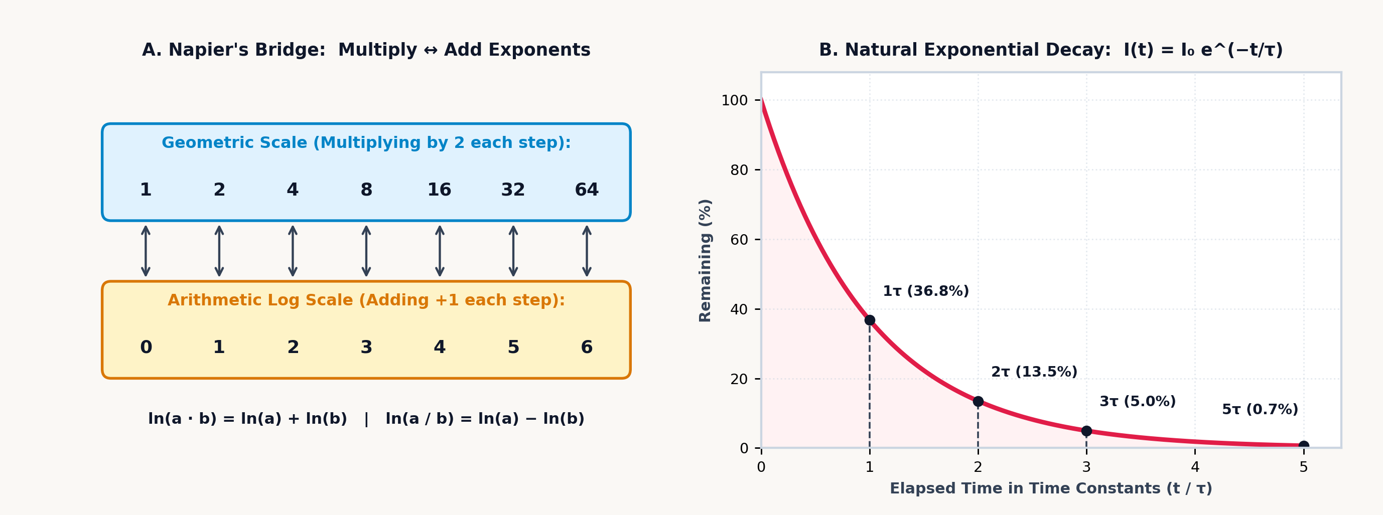
Napier set out to construct a mapping in mathematics that converts multiplication into addition, division into subtraction, and square or cube root extraction into division by \(2\) or \(3\). Aligning a row of integer exponents above the corresponding powers of three and powers of ten reveals the underlying isomorphism:
| Arithmetic Exponent (\(n\)) | \(0\) | \(1\) | \(2\) | \(3\) | \(4\) | \(5\) | \(6\) | \(7\) |
|---|---|---|---|---|---|---|---|---|
| Ternary Power (\(3^n\)) | \(1\) | \(3\) | \(9\) | \(27\) | \(81\) | \(243\) | \(729\) | \(2{,}187\) |
| Decimal Power (\(10^n\)) | \(1\) | \(10\) | \(100\) | \(1{,}000\) | \(10{,}000\) | \(100{,}000\) | \(10^6\) | \(10^7\) |
To multiply \(27 \times 81\) via powers of three, match each factor to its exponent: \(27 = 3^3\) corresponds to \(n = 3\), and \(81 = 3^4\) corresponds to \(n = 4\). Adding their exponents (\(3 + 4 = 7\)) points to \(3^7 = 2,187\) (\(27 \times 81 = 2,187\)). That correspondence holds for any positive base \(b\) because an exponent counts repeated factors of the base:
Napier spent twenty years interpolating the continuous values between the integers through a kinematic model of two points moving in tandem along straight lines. The first point (the logarithm track) travels along an infinite straight line at a uniform velocity \(v_0\), covering equal arithmetic increments of distance in equal intervals of time (\(0, \Delta x, 2\Delta x, 3\Delta x, \dots\)). Over the same time intervals, the second point (the number track) starts at distance \(L\) from a terminal mark and moves toward it at a speed proportional to the distance remaining, covering equal geometric ratios in equal intervals of time (\(L, L r, L r^2, L r^3, \dots\)).
By pairing the arithmetic position of the first point with the geometric position of the second point at every instant, Napier established a continuous correspondence between addition and multiplication. In differential notation, Napier's first point obeys \(\frac{dx}{dt} = v_0\) so that \(x(t) = v_0 t\), while his second point starts at \(y(0) = L = 10^7\) (the radius of a seventeenth-century trigonometric sine table accurate to seven figures) and decelerates in proportion to its remaining distance from the origin:
More than a century before the natural base \(e\) was formalized, Napier's kinematic definition had implicitly constructed a table of natural logarithms scaled by \(10^7\). In 1614, he published his logarithmic tables (Napier, 1614), coining the word logarithm from the Greek logos ("ratio") and arithmos ("number") to signify the number that counts ratios. A year later, London geometry professor Henry Briggs traveled to Edinburgh and worked with Napier to normalize logarithms to base \(10\), where \(\log_{10} 1 = 0\), \(\log_{10} 10 = 1\), \(\log_{10} 100 = 2\), and \(\log_{10} 1000 = 3\).
For any two positive numbers \(a\) and \(b\), Napier and Briggs's logarithmic function satisfies three structural identities together with the universal change-of-base identity:
Because \(b^{\log_b x} = x\) by definition, taking the natural or base-\(10\) logarithm of both sides gives \(\log_b(x)\cdot\ln b = \ln x\), proving that a logarithm in any positive base \(b \ne 1\)—including base-\(2\) information entropy \(\log_2(x) = \frac{\ln x}{\ln 2}\) in bits—is the ratio of two natural or common logarithms, and that a telescoping product across stepping bases collapses to its endpoints (\(\log_2 3 \cdot \log_3 4 \cdot \log_4 5 \cdots \log_{63} 64 = \frac{\ln 64}{\ln 2} = \mathbf{6}\)). Where multiplying two eight-digit numbers by hand once took twenty minutes, an astronomer could look up their two logarithms in Briggs's table, add them in seconds, and read the antilogarithm matching that sum (Figure 3.1). Extracting a cube root (\(\sqrt[3]{y} = y^{1/3}\)) reduced to looking up \(\log y\) and dividing by \(3\). By replacing multi-digit multiplication with addition, logarithms doubled the working life of scientists across astronomy, navigation, and engineering.
Physical CPA Studio Bridge (
Book 4 Units 02–04— Algebra Tile L-Frame & Prime Factor Studio):
In the companion StackCalc High School & STEM Lab (Book 4), students build these two algebraic and logarithmic transformations with their hands before evaluating them on the SC-32 stack. In Units 02–03, Al-Khwarizmi's geometric completing-the-square derivation (\(x^2 + bx = (x + b/2)^2 - (b/2)^2\)) is modeled inside the \(36\text{ mm} \times 36\text{ mm}\) Algebra Tile \(90^\circ\) Corner L-Frame by splitting the linear \(bx\) strip into two symmetric \((b/2)x\) wings around the \(x^2\) flat and measuring the missing \((b/2)^2\) corner square. In Unit 04, Napier's multiplication-to-addition isomorphism is realized physically in the Prime Factor Logarithmic Tower Studio (PRIME-01), where each prime block \(p \in \{2, 3, 5, 7, \dots\}\) is 3D-printed to an exact logarithmic height \(h(p) = 7.0 \cdot \log_2(p)\text{ mm}\) (\(h(2) = 7.00\text{ mm}\), \(h(3) = 11.09\text{ mm}\), \(h(5) = 16.25\text{ mm}\)): stacking Prime \(2\) on Prime \(3\) physically adds their heights (\(7.00 + 11.09 = 18.09\text{ mm}\)) to align flush with the \(2 \times 3 = 6\) tick mark on the logarithmic comparator stage.
To evaluate any logarithm to 16 digits without storing Briggs's thousand-page book in memory, the SC-32 uses binary floating-point range reduction (Cody & Waite, 1980), factoring any positive number \(x = m \cdot 2^k\) into its normalized binary significand \(m \in [\frac{1}{\sqrt{2}}, \sqrt{2})\) near \(1\) and its exact integer binary exponent \(k\):
Because \(m\) is confined to a narrow interval around \(1\), the natural logarithm \(\ln(m)\) can be expanded in terms of the rapidly converging rational transformation \(z = \frac{m - 1}{m + 1}\):
which converges to 16 decimal digits in a small number of odd powers. Unlike the naive Taylor series \(\ln(1 + u) = u - u^2/2 + u^3/3 - \dots\), which diverges for \(u > 1\) and converges slowly near \(u = 1\), the bilinear mapping \(z = \frac{m - 1}{m + 1}\) compresses the reduced binary interval \(m \in [1/\sqrt{2}, \sqrt{2})\) onto \(|z| \le \frac{\sqrt{2} - 1}{\sqrt{2} + 1} = 3 - 2\sqrt{2} \approx 0.172\), so each successive odd power \(z^{2n+1}\) shrinks by at least \(z^2 \le 17 - 12\sqrt{2} \approx 2.94 \times 10^{-2}\) (more than \(1.5\) decimal digits per term). For \(x = 10 = 1.25 \times 2^3\) (\(m = 1.25\), \(k = 3\)), the bilinear variable reduces to the simple fraction \(z = \frac{1.25 - 1}{1.25 + 1} = \frac{1}{9}\).
3.1.1 Logarithmic Perception and Decibel Scaling
Napier and Briggs's base-10 logarithm extends well beyond computational tables because physical waves and human sensory systems span many orders of magnitude. In a dark room illuminated by a single candle, introducing a second candle doubles the photon flux and produces an unmistakable increase in perceived brightness. In a hall already illuminated by \(100\) candles, introducing a \(101\text{st}\) candle changes the stimulus by only one percent, and the increment is imperceptible. Sensory receptors scale with the relative ratio (\(\frac{\text{new intensity}}{\text{old intensity}}\)), not the additive increment (\(+1\text{ candle}\)): each tenfold multiplication of physical energy produces one equal perceptual step.
Four standard measurement scales in acoustics, geophysics, astrophysics, and radio engineering apply this base-10 logarithmic compression, mapping dimensionless physical ratios across powers of ten. In acoustics, the faintest pressure fluctuation detectable by the human eardrum has a root-mean-square amplitude of \(p_0 = 20\,\mu\text{Pa}\) (\(2 \times 10^{-5}\text{ Pa}\)), while a nearby jet engine reaches \(20\text{ Pa}\). Between those extremes, acoustic pressure spans a million-fold range (\(10^6:1\)) and acoustic intensity \(I \propto p^2\) spans twelve orders of magnitude (\(10^{12}:1\)). Along the inner ear, the tapered basilar membrane of the mammalian cochlea maps those twelve orders of magnitude onto the \(0\text{ to }120\text{ dB}\) Sound Pressure Level scale:
For a stadium acoustic wave of root-mean-square pressure \(p_{\text{rms}} = 1.45\text{ Pa}\) referenced to the \(p_0 = 2 \times 10^{-5}\text{ Pa}\) cochlear hearing threshold, the ratio \(p_{\text{rms}} / p_0\) shows that the wave amplitude is \(72,500\times\) the threshold of hearing. Taking the base-10 logarithm compresses that \(72,500:1\) pressure ratio into \(\approx 4.86\) decades of amplitude, and scaling by \(20\) (since acoustic intensity scales as \(p^2\)) yields \(\approx \mathbf{97.207\text{ dB SPL}}\) (\(\approx 9.721\text{ Bels}\); a \(p_{\text{rms}} = 2\text{ Pa}\) wave at \(10^5 p_0\) reaches \(\mathbf{100\text{ dB SPL}}\)). In architectural acoustics, a \(60\text{ dB}\) (\(10^6:1\)) drop in energy density sets the \(0.161\text{ s/m}\) Sabine reverberation factor across a concert hall of volume \(V = 4,500\text{ m}^3\) and absorption area \(A = 320\text{ sabins}\) (\(\text{m}^2\)), yielding a reverberation decay time of \(T_{60} = 0.161 V / A \approx \mathbf{2.264\text{ s}}\).
When that same wave energy radiates through the solid Earth or across interstellar space, two further base-10 logarithmic scales govern geophysics and observational astronomy. In seismology, Charles Richter originally defined local earthquake magnitude \(M_L = \log_{10}(A/A_0)\) by comparing the peak trace amplitude \(A\) recorded on a standard Wood–Anderson torsion seismograph against a reference threshold amplitude \(A_0\). To measure giant subduction ruptures without instrument saturation, Hiroo Kanamori and Thomas Hanks linked earthquake size directly to the physical fault mechanics through the seismic moment \(M_0 = \mu A_{\text{fault}} D\) (in \(\text{N}\cdot\text{m}\))—the product of the crustal rock's shear modulus \(\mu\), the ruptured fault surface area \(A_{\text{fault}}\), and the average slip displacement \(D\) across the fault—defining the Moment Magnitude \(M_w = \frac{2}{3}\log_{10} M_0 - 6.07\) and the radiated elastic wave energy \(E_s\) (in joules) via \(\log_{10}(E_s/\text{J}) = 1.5 M_w + 4.8\). Because \(M_w\) multiplies \(\log_{10} M_0\) by \(\frac{2}{3}\) while \(\log_{10} E_s\) scales \(M_w\) by \(1.5 = \frac{3}{2}\), each integer step up the magnitude scale corresponds to a tenfold increase in ground-motion amplitude \(A\) and a \(10^{1.5} = 10\sqrt{10} \approx \mathbf{31.623\times}\) increase in radiated elastic wave energy \(E_s\); a two-unit jump from a \(M_w = 7\) earthquake to a \(M_w = 9\) megathrust rupture multiplies released energy by \(10^{1.5 \times 2} = \mathbf{1,000\times}\).
In observational astronomy, N. R. Pogson's stellar magnitude scale relates apparent magnitudes \(m_1, m_2\) to irradiance flux via \(m_1 - m_2 = -2.5\log_{10}(F_1/F_2)\), where a 5-magnitude span corresponds to a \(100\times\) (\(10^2\)) ratio in photon flux and each unit step represents a flux ratio of \(100^{1/5} = 10^{0.4} \approx \mathbf{2.512\times}\). Comparing Sirius (\(m_1 = -1.46\)) against Vega (\(m_2 = +0.03\)) via \(F_1/F_2 = 10^{-0.4(m_1 - m_2)}\) shows that Sirius delivers \(\approx \mathbf{3.945\times}\) Vega's photon flux, while combining apparent magnitude \(m = 1.25\) and absolute magnitude \(M = -8.38\) for the supergiant Deneb in the distance modulus \(d = 10 \times 10^{(m - M)/5}\text{ pc}\) gives a heliocentric distance of \(d \approx \mathbf{843.335\text{ parsecs}}\).
A coherent spacecraft radio carrier completes the quartet of base-10 wave-attenuation scales. When an isotropic transmitting antenna radiates electromagnetic power \(P_t\) at carrier frequency \(f\) (wavelength \(\lambda = c/f\), where \(c\) is the vacuum speed of light) across a vacuum link of distance \(d\), the outgoing wavefront spreads over a spherical shell of surface area \(4\pi d^2\), while an isotropic receiving antenna intercepts that flux over an effective diffraction capture area of \(\lambda^2 / (4\pi) = c^2 / (4\pi f^2)\). Multiplying those two geometric factors gives Friis's free-space power transmission ratio \(\frac{P_r}{P_t} = \left(\frac{c}{4\pi d f}\right)^2\) for the received power \(P_r\), and inverting that ratio into the attenuation loss \(P_t / P_r = \left(\frac{4\pi d f}{c}\right)^2\) converts via Napier's product rule into the decibel Free-Space Path Loss (FSPL):
Squaring the distance-frequency product \(\frac{4\pi d f}{c}\) pulls a factor of \(2\) in front of \(10\log_{10}\) to make each coefficient \(20\), while Napier's product rule splits the total attenuation into three additive decibel terms: spherical spreading loss \(20\log_{10}(d)\), receiving-aperture shrinkage \(20\log_{10}(f)\) at shorter wavelengths, and the constant baseline \(20\log_{10}(4\pi / c) \approx -147.552\text{ dB}\). For a \(f = 2.4\text{ GHz}\) (\(2.4 \times 10^9\text{ Hz}\)) spacecraft telemetry link across \(d = 10\text{ km}\) (\(10,000\text{ m}\)), free-space path loss adds \(20\log_{10}(10,000) = 80\text{ dB}\) and \(20\log_{10}(2.4 \times 10^9) \approx 187.604\text{ dB}\) to \(-147.552\text{ dB}\) to yield \(\text{FSPL} \approx \mathbf{120.052\text{ dB}}\).
3.1.2 Acidity, Arterial Blood Gases, and Excitable Membranes
Across aqueous, electrochemical, and physiological systems, logarithmic scales arise from the statistical mechanics of thermal motion: because the Gibbs chemical potential of a dissolved species grows with the logarithm of its thermodynamic activity (\(\mu = \mu^\circ + RT\ln a\)), equilibrium proton transfer, galvanic cell voltage, and membrane ion transport all reduce to logarithmic ratios.
In aqueous chemistry, the \(\text{pH}\) scale maps fourteen orders of magnitude of hydronium ion molarity \([\text{H}_3\text{O}^+]\) (\(\text{mol/L}\)) onto a linear scale from \(0\) (concentrated strong acid) to \(14\) (concentrated strong base), centered at \(\text{pH} = 7\) for neutral pure water at \(25^\circ\text{C}\) where \(K_w = [\text{H}_3\text{O}^+][\text{OH}^-] = 10^{-14}\):
Because base-10 logarithm and base-10 exponentiation are exact mathematical inverses, converting hydronium concentration to \(\text{pH}\) and inverting \(\text{pH}\) back to molar concentration mirror one another: for \([\text{H}_3\text{O}^+] = 4.2 \times 10^{-5}\text{ mol/L}\), \(-\log_{10}(4.2 \times 10^{-5}) \approx \mathbf{4.377}\). When a weak acid \(\text{HA}\) of dissociation constant \(\text{pK}_a = -\log_{10} K_a\) is mixed with its conjugate base salt \(\text{A}^-\), the Henderson–Hasselbalch buffer equation shows that equimolar concentrations (\([\text{A}^-] = [\text{HA}]\)) make \(\log_{10}(1) = 0\) and fix \(\text{pH} = \text{pK}_a\) at maximum buffer capacity. For an acetic acid buffer (\(\text{pK}_a = 4.76\)) pairing \([\text{A}^-] = 0.185\text{ M}\) with \([\text{HA}] = 0.12\text{ M}\), the log ratio \(\log_{10}(0.185 / 0.12) \approx +0.188\) shifts the solution to \(\text{pH} \approx \mathbf{4.948}\). In pulmonary and critical-care medicine, the carbonic acid–bicarbonate buffer maintains arterial blood plasma near \(\text{pH } 7.4\) (\(\text{pK}_a = 6.1\), dissolved \(\text{CO}_2\) solubility \(\alpha = 0.0301\text{ mmol/(L}\cdot\text{mmHg)}\)):
For an arterial blood-gas panel showing serum bicarbonate \([\text{HCO}_3^-] = 24\text{ mmol/L}\) and partial pressure \(P_{\text{CO}_2} = 40\text{ mmHg}\), dividing \([\text{HCO}_3^-]\) by the dissolved carbonic acid denominator \(0.0301 \times 40 = 1.204\text{ mmol/L}\) gives a \(\approx 19.934:1\) base-to-acid ratio whose base-10 logarithm yields \(\text{pH} \approx \mathbf{7.4}\), corresponding to an effective free hydronium concentration of \(10^{-7.4} \times 10^9 \approx \mathbf{39.811\text{ nmol/L}}\) (or \(10^{-\text{pH}} \times 10^9 \approx \mathbf{39.849\text{ nmol/L}}\) from the unrounded logarithm).
When chemical species transfer \(n\) moles of electrons per formula unit across an electrode interface at absolute temperature \(T\) (with molar gas constant \(R \approx 8.314\text{ J/(mol}\cdot\text{K)}\) and Faraday's constant \(F = N_A e \approx 96,485.332\text{ C/mol}\)), the Gibbs free-energy change \(\Delta G = \Delta G^\circ + RT\ln Q\) equates directly to electrical work \(-nFE\). Dividing by \(-nF\) links the standard reduction potential \(E^\circ = -\Delta G^\circ/(nF)\), the live reaction quotient \(Q\), and the thermodynamic equilibrium constant \(K\) through the Nernst electrochemical equation:
Scarce product ions (\(Q < 1\)) make \(\ln Q\) negative and boost the live cell voltage \(E\) above its standard baseline \(E^\circ\); as reactants are consumed and products accumulate during discharge, \(Q\) climbs toward the equilibrium constant \(K = \exp(nFE^\circ / RT)\), raising the thermal-voltage penalty \(\frac{RT}{nF}\ln Q\) until \(\frac{RT}{nF}\ln K = E^\circ\) and \(E\) reaches zero in a spent battery. For a two-electron Daniell cell (\(E^\circ = 1.1\text{ V}, T = 298.15\text{ K}, n = 2\)) at reaction quotient \(Q = [\text{Zn}^{2+}]/[\text{Cu}^{2+}] = 0.015\), the natural logarithm \(\ln(0.015) \approx -4.2\) scaled by the two-electron thermal voltage \(RT/(nF) \approx 0.013\text{ V}\) (\(12.846\text{ mV}\)) produces a shift of \(\approx -0.054\text{ V}\) and a net galvanic cell potential of \(E \approx \mathbf{1.154\text{ V}}\).
Across excitable biological membranes, a single-ion Nernst potential like potassium's \(E_{\text{K}} = \frac{RT}{F}\ln\frac{[\text{K}^+]_o}{[\text{K}^+]_i}\) applies only when one ion species can cross the membrane. A living neuron's lipid bilayer, however, is pierced by protein ion channels with distinct relative membrane permeabilities \(P_{\text{K}}, P_{\text{Na}},\) and \(P_{\text{Cl}}\) that simultaneously pass potassium (\(\text{K}^+\)), sodium (\(\text{Na}^+\)), and negatively charged chloride (\(\text{Cl}^-\)) between the extracellular fluid (subscript \(o\) for outside) and intracellular cytoplasm (subscript \(i\) for inside). Weighing each ion's concentration gradient by its channel permeability yields the Goldman–Hodgkin–Katz (GHK) voltage equation for the resting transmembrane potential \(V_m\):
All three ions pull on the membrane voltage in proportion to their channel permeabilities: whichever ion has the largest \(P\) dominates the ratio and draws \(V_m\) toward its own single-ion Nernst potential. Chloride's concentrations appear inverted relative to the cations—intracellular \([\text{Cl}^-]_i\) grouped with the extracellular cations above the line and extracellular \([\text{Cl}^-]_o\) grouped with the intracellular cations below—because chloride carries a negative charge (\(z = -1\)), and negating a logarithm inverts its argument (\(\ln(a/b)^{-1} = \ln(b/a)\)). Whereas a mammalian neuron permeable only to potassium (\([\text{K}^+]_o = 4\text{ mM}\), \([\text{K}^+]_i = 140\text{ mM}\)) would rest near its potassium reversal potential of \(-95\text{ mV}\), a living resting membrane also admits a slight inward trickle of concentrated extracellular sodium (\(P_{\text{K}} : P_{\text{Na}} : P_{\text{Cl}} = 1 : 0.04 : 0.45\)), depolarizing the resting potential toward \(-75\text{ mV}\).
Two companion equilibrium relations govern electrostatic ion shielding in solution and oxygen transport in blood. In concentrated electrolyte solutions where each dissolved ion species \(i\) has molar concentration \(c_i\) and integer charge valence \(z_i\), electrostatic attraction gathers a screening cloud of opposite counter-ions around every charge; the total electrical crowding of the solution is measured by its ionic strength \(I_c\), which depresses the mean ionic activity coefficient \(\gamma_{\pm}\) of a salt with cation/anion valences \(z_+, z_-\) according to the Debye–Hückel limiting law (with solvent constant \(A_{\text{DH}}\)). Meanwhile, in respiratory physiology, a tetrameric hemoglobin molecule with \(n\) cooperative binding sites and half-saturation oxygen pressure \(P_{50}\) binds dissolved oxygen at partial pressure \(P_{\text{O}_2}\) to reach fractional saturation \(\theta\) under the Hill oxygen-binding isotherm \(\theta = \frac{P_{\text{O}_2}^n}{P_{50}^n + P_{\text{O}_2}^n}\) (which divides top and bottom by \(P_{\text{O}_2}^n\) so \(P_{\text{O}_2}\) appears only once):
Squaring the charge valence \(z_i^2\) in the ionic strength \(I_c\) gives multivalent ions outsized influence—a divalent \(\text{Ca}^{2+}\) ion (\(z^2 = 4\)) contributes four times the electrostatic screening of a monovalent \(\text{Na}^+\) ion (\(z^2 = 1\))—while the negative \(-\sqrt{I_c}\) dependence lowers \(\gamma_{\pm}\) as denser counter-ion clouds shield dissolved ions from one another. Hemoglobin's cooperative exponent \(n = 2.8\) turns \((P_{50}/P_{\text{O}_2})^n\) into a steep molecular switch around \(P_{50}\): in the lungs where \(P_{\text{O}_2} \gg P_{50}\), raising \(P_{50}/P_{\text{O}_2} < 1\) to the \(2.8\) power drives the ratio near zero so \(\theta \to 1\) (nearly \(100\%\) loaded), whereas in working muscle where \(P_{\text{O}_2}\) falls below \(P_{50}\), \((P_{50}/P_{\text{O}_2})^n\) climbs rapidly above \(1\) to release bound oxygen. For \(0.01\text{ M}\) aqueous calcium chloride (\(\text{CaCl}_2 \to \text{Ca}^{2+} + 2\text{Cl}^-\), with \(I_c = \frac{1}{2}[0.01(2^2) + 0.02(1^2)] = 0.03\text{ M}\) and water Debye–Hückel constant \(A_{\text{DH}} = 0.509\text{ M}^{-1/2}\) at \(25^\circ\text{C}\)), the mean ionic activity coefficient is \(\gamma_{\pm} = 10^{-0.509(2)\sqrt{0.03}} \approx \mathbf{0.666}\), while tetrameric hemoglobin (\(P_{50} = 26\text{ mmHg}\), \(n = 2.8\)) at alveolar oxygen tension \(P_{\text{O}_2} = 100\text{ mmHg}\) reaches \(\theta = [1 + (26/100)^{2.8}]^{-1} \approx \mathbf{97.75\%}\) fractional saturation.
3.2 Fractional Power Laws and the Natural Base of Change
Once Napier established that \(\log(y^x) = x\log y\), raising any positive real number \(y > 0\) to an arbitrary real exponent \(x\) followed from composing the natural logarithm and exponential:
On a four-register operational stack, powers, roots, and reciprocals divide naturally into two structural classes: in-place unary transformations (\(x^2\), \(\sqrt{x}\), and \(1/x\)) that transform Register \(X\) in place without disturbing values held in Registers \(Y, Z,\) or \(T\), and two-register dyadic operations that combine Register \(Y\) with Register \(X\) (raising base \(Y\) to exponent \(X\) as \(Y^X\), extracting the \(X\)-th root of \(Y\) as \(Y^{1/X}\), and evaluating the parallel harmonic product-over-sum \(\frac{YX}{Y+X}\)).
3.2.1 Planets, Mice, Whales, and the Harmonic Operator
Fractional exponents—\(y^{2/3}\), \(y^{3/4}\), \(y^{1.32}\), and \((1 - \beta^2)^{-1/2}\)—govern scaling laws across celestial mechanics, physiology, and special relativity. Under Kepler's Third Law of planetary motion, the square of a planet's orbital period \(T\) (in Earth years) equals the cube of its semi-major axis \(a\) (in Astronomical Units, where \(1\text{ AU}\) is the mean Earth–Sun distance). Equating gravitational attraction \(G M_{\odot} m / a^2\) with centripetal force \(m v^2 / a = m(2\pi a / T)^2 / a\) yields \(T^2 = \frac{4\pi^2}{G M_{\odot}} a^3\), and taking the cube root of both sides expresses \(T^2 = a^3\) as a \(2/3\) fractional power law:
Under the fractional-power law \(a = \sqrt[3]{T^2}\), Mars's sidereal period \(T \approx 1.881\text{ yr}\) (\(T^2 \approx 3.537\text{ yr}^2\)) yields a semi-major axis of \(a \approx \mathbf{1.524\text{ AU}}\), while Halley's Comet (\(T = 75.32\text{ yr}\), \(T^2 \approx 5,673.1\text{ yr}^2\)) stretches out to a semi-major axis of \(a \approx \mathbf{17.835\text{ AU}}\) beyond the orbit of Uranus.
A second fractional power law governs comparative physiology. Plotting basal metabolic rate \(B\) (in Watts or kilocalories per day) against body mass \(M\) across homeothermic mammals ranging from a \(20\text{-gram}\) mouse to a \(4,000\text{-kilogram}\) elephant (\(200,000\times\) more massive) reveals that metabolic rate scales neither linearly with mass (\(M^1\)) nor with Euclidean exterior surface area (\(M^{2/3} \approx M^{0.67}\)), but follows Kleiber's three-quarters power law:
This \(3/4\) exponent emerges because biological vascular and bronchial trees are space-filling fractal networks that minimize hydrodynamic pumping work across three spatial dimensions, introducing an effective fourth scaling dimension (\(3 / (3 + 1) = 3/4\)). Because basal metabolism scales as \(M^{0.75}\) (with mammalian constant \(B_0 = 70\text{ kcal/(day}\cdot\text{kg}^{0.75}\text{)}\)), an Asian elephant of mass \(M = 4,000\text{ kg}\) requires \(70 \times 4000^{0.75} \approx \mathbf{35,208.136\text{ kcal/day}}\) (\(\approx 8.802\text{ kcal/kg}\), compared with \(\approx \mathbf{124.48\text{ kcal/kg}}\) for a \(0.1\text{ kg}\) rodent), while mammalian resting heart rate scales inversely as \(f_H \approx 241 M^{-0.25}\text{ bpm}\) (\(\approx \mathbf{30.304\text{ bpm}}\) at \(M = 4,000\text{ kg}\)).
A negative half-integer power law governs relativistic particle kinematics. In Earth's stratosphere, \(15\text{ kilometers}\) (\(15,000\text{ meters}\)) above sea level, primary cosmic rays collide with atmospheric nuclei and produce unstable secondary muons. In its rest frame, a muon decays with a mean proper lifetime of \(\tau_0 \approx 2.197\text{ microseconds}\) (\(2.197 \times 10^{-6}\text{ s}\)). Even for a muon descending at \(99.5\%\) of the speed of light (\(\beta = v/c = 0.995\)), classical kinematics predicts a mean propagation distance of only \(d_{\text{classical}} = \beta c \tau_0 \approx \mathbf{655.351\text{ meters}}\) before decay—far too short to reach sea-level detectors \(15,000\text{ meters}\) below.
By invariance of the spacetime interval \(c^2 \Delta\tau^2 = c^2 \Delta t^2 - \Delta x^2\) across inertial frames, relativistic time dilation stretches the laboratory lifetime \(\Delta t = \gamma \Delta\tau\) according to the Lorentz factor \(\gamma = (1 - \beta^2)^{-1/2}\). At \(\beta = 0.85\), relativistic time dilation stretches the laboratory clock by \(\gamma \approx \mathbf{1.898}\); at \(\beta = 0.995\), \(\gamma\) reaches \(\approx \mathbf{10.013}\), extending the muon's mean laboratory decay path tenfold to \(d = \gamma \beta c \tau_0 \approx \mathbf{6,561.715\text{ meters}}\) so a substantial fraction survives to sea level.
Built on the parallel reciprocal law (\(\frac{1}{T} = \frac{1}{T_1} + \frac{1}{T_2}\)), the product-over-sum harmonic operator \(x \parallel y = \frac{x \cdot y}{x + y} = \left(\frac{1}{x} + \frac{1}{y}\right)^{-1}\) unifies five distinct domains of physics and engineering:
| Physical Domain | What Combines via \(x \parallel y = \frac{x y}{x + y}\) | Why the Reciprocal-Sum Law Appears |
|---|---|---|
| 1. Parallel Electrical Resistors | \(R_{\text{eq}} = R_1 \parallel R_2 = \frac{R_1 R_2}{R_1 + R_2}\) | Both resistors share the same voltage \(V\), while their currents (\(I_i = V/R_i\)) add. |
| 2. Thin Optical Lenses & Mirrors | \(f = d_o \parallel d_i = \frac{d_o d_i}{d_o + d_i}\) | Light rays from object distance \(d_o\) bend by constant optical power \(1/f\) to focus at image distance \(d_i\) (\(\frac{1}{f} = \frac{1}{d_o} + \frac{1}{d_i}\)). |
| 3. Capacitors Wired in Series | \(C_{\text{eq}} = C_1 \parallel C_2 = \frac{C_1 C_2}{C_1 + C_2}\) | Series capacitor plates trap the same charge \(Q\), while their voltage drops (\(V_i = Q/C_i\)) add. |
| 4. Mechanical Springs in Series | \(k_{\text{eq}} = k_1 \parallel k_2 = \frac{k_1 k_2}{k_1 + k_2}\) | Two springs hooked end-to-end feel the same tension force \(F\), while their stretches (\(\Delta x_i = F/k_i\)) add. |
| 5. Round-Trip Average Speed | \(v_{\text{avg}} = 2(v_1 \parallel v_2) = \frac{2 v_1 v_2}{v_1 + v_2}\) | Driving \(D\text{ miles}\) uphill at \(v_1 = 30\text{ mph}\) and \(D\text{ miles}\) downhill at \(v_2 = 60\text{ mph}\) adds times (\(D/v_1 + D/v_2\)) to give \(2(30 \parallel 60) = \mathbf{40\text{ mph}}\) (not \(45\text{ mph}\)). |
All five systems reduce to \(x \parallel y\) because each pairs a shared quantity across elements with an additive reciprocal conductance, vergence, elastance, compliance, or transit rate. Because \(x \parallel y\) is both commutative (\(x \parallel y = y \parallel x\)) and associative (\((x \parallel y) \parallel z = x \parallel (y \parallel z)\)), three or more branches fold across Registers \(Y\) and \(X\) just like addition or multiplication: a three-branch resistor bank \(120\,\Omega \parallel 180\,\Omega \parallel 360\,\Omega\) folds to \(\mathbf{60\,\Omega}\), a Gaussian thin lens at \(d_o = 30\text{ cm}\) and \(d_i = 15\text{ cm}\) has focal length \(f = 30 \parallel 15 = \mathbf{10\text{ cm}}\), and doubling \(30 \parallel 60\) gives the harmonic mean round-trip speed of \(\mathbf{40\text{ mph}}\).
3.2.2 The Natural Base \(e\), Radiocarbon Clocks, and Thermal Activation Barriers
Whereas Briggs's base-10 logarithm steps by discrete powers of ten, continuous growth and decay processes unfold along the natural base \(e\):
In mathematical analysis, \(e^x\) (eˣ) and its inverse \(\ln x\) form the natural exponential and logarithm because term-by-term differentiation of the factorial power series maps each term \(\frac{x^k}{k!}\) to \(\frac{k x^{k-1}}{k!} = \frac{x^{k-1}}{(k-1)!}\), reproducing the series unchanged:
Radiometric dating applies natural logarithmic decay inversion to determine the age of organic archaeological specimens and geological strata. Once an organism dies, its trapped carbon-14 (\(^{14}\text{C}\)) nuclei undergo beta decay back into nitrogen-14 with a half-life of \(t_{1/2} = 5,730\text{ years}\):
For an Ice Age hearth bone retaining \(23.4\%\) of its original \({}^{14}\text{C}\) (\(N/N_0 = 0.234\), \(t_{1/2} = 5,730\text{ yr}\)), the natural logarithm \(\ln(0.234) \approx -1.452\) divided by \(-\ln(2) \approx -0.693\) reveals that \(\approx 2.095\) half-lives have elapsed, establishing an age of \(\approx \mathbf{12,006.754\text{ years}}\). For Precambrian volcanic basalt billions of years old, potassium–argon dating (\(t = \frac{1}{\lambda}\ln\left(1 + C\frac{^{40}\text{Ar}}{^{40}\text{K}}\right)\) with \(^{40}\text{Ar}/{}^{40}\text{K} = 0.085\), branching factor \(C = 9.54\), and decay constant \(\lambda = 5.543 \times 10^{-10}\text{ yr}^{-1}\)) dates the solidification of the rock to \(\approx \mathbf{1.071 \times 10^9\text{ years}}\) (\(\approx 1.071\text{ billion years}\)), while at an annual compound growth rate of \(r = 7.2\%\), the ratio \(\ln(2) / \ln(1.072) \approx 0.693 / 0.07\) gives a doubling time of \(\approx \mathbf{9.97\text{ years}}\). The same first-order exponential relaxation governs macroscopic heat transfer and RC electrical networks (\(\Delta T(t) = \Delta T_0 e^{-t/\tau} \implies t = -\tau \ln(\Delta T(t)/\Delta T_0)\)): an RC timing network with resistance \(R = 150\text{ k}\Omega\) and capacitance \(C = 47\,\mu\text{F}\) (time constant \(\tau = RC = 7.05\text{ s}\)) decays to \(10\%\) (\(0.1\)) of its initial step voltage after \(-\tau\ln(0.1) \approx \mathbf{16.233\text{ seconds}}\).
Across chemical kinetics, solid-state metallurgy, phase equilibrium, atmospheric physics, and semiconductor junctions, thermal processes share a single statistical foundation: in a reservoir at absolute temperature \(T\), the probability that random thermal collisions concentrate an energy \(\Delta E\) onto a single molecule or lattice site decays exponentially as the Boltzmann factor \(\exp(-\Delta E / k_B T)\) (or \(\exp(-\Delta E / RT)\) per mole). Under the Arrhenius rate law, a chemical reaction rate constant \(k = A\exp(-E_a / RT)\) equals the molecular collision frequency \(A\) multiplied by the Boltzmann fraction exceeding the activation barrier \(E_a\).
For an enzymatic or organic reaction with \(A = 1.25 \times 10^{11}\text{ s}^{-1}\) and \(E_a = 65,000\text{ J/mol}\) at \(T = 310\text{ K}\) (\(R \approx 8.314\text{ J/(mol}\cdot\text{K)}\)), only about one molecular oscillation in \(9 \times 10^{10}\) surmounts the barrier, giving \(k \approx \mathbf{1.395\text{ s}^{-1}}\). In the inverse problem, comparing rate constants measured at two temperatures (\(k_1 = 3.25 \times 10^{-4}\text{ s}^{-1}\) at \(T_1 = 300\text{ K}\) and \(k_2 = 2.85 \times 10^{-2}\text{ s}^{-1}\) at \(T_2 = 350\text{ K}\)) via \(E_a = \frac{R\ln(k_2/k_1)}{1/T_1 - 1/T_2}\) divides the logarithmic rate ratio \(R\ln(k_2/k_1) \approx \mathbf{37.198\text{ J/(mol}\cdot\text{K)}}\) by the reciprocal temperature span \(1/300 - 1/350 \approx 4.76 \times 10^{-4}\text{ K}^{-1}\) to recover the activation barrier \(E_a \approx \mathbf{78.115\text{ kJ/mol}}\).
The same thermal barrier governs atomic hopping in solids and phase transitions in liquids. When interstitial carbon atoms diffuse through austenite steel inside a \(T = 1,200\text{ K}\) heat-treating furnace, an atom can hop to a neighboring lattice site only when thermal vibration supplies the molar diffusion activation energy \(Q = 148,000\text{ J/mol}\); scaling the high-temperature pre-exponential diffusivity \(D_0 = 2.3 \times 10^{-5}\text{ m}^2/\text{s}\) by the Boltzmann jump fraction \(\exp(-Q/RT)\) (where \(Q/(RT) \approx 14.834\) and \(\exp(-14.834) \approx 3.61 \times 10^{-7}\) for \(R \approx 8.314\text{ J/(mol}\cdot\text{K)}\)) yields a solid-state diffusivity of \(D = D_0\exp(-Q/RT) \approx \mathbf{8.31 \times 10^{-12}\text{ m}^2/\text{s}}\). Along a liquid–vapor coexistence curve, escaping from the liquid phase requires overcoming the molar enthalpy of vaporization \(\Delta H_{\text{vap}}\), so the Clausius–Clapeyron relation relates equilibrium vapor pressures \(P_1, P_2\) at absolute temperatures \(T_1, T_2\) via \(P_2 = P_1 \exp[-\frac{\Delta H_{\text{vap}}}{R}(\frac{1}{T_2} - \frac{1}{T_1})]\): cooling water from its sea-level boiling point of \(100^\circ\text{C}\) (\(T_1 = 373.15\text{ K}\), \(P_1 = 101.325\text{ kPa}\), \(\Delta H_{\text{vap}} = 40,660\text{ J/mol}\)) to \(60^\circ\text{C}\) (\(T_2 = 333.15\text{ K}\)) increases the reciprocal temperature difference \(1/T_2 - 1/T_1 \approx 3.22 \times 10^{-4}\text{ K}^{-1}\) and drops the equilibrium vapor pressure to \(P_2 \approx \mathbf{21.006\text{ kPa}}\).
Even in a planetary gravitational field or across a crystalline semiconductor bandgap, the Boltzmann factor sets the equilibrium distribution. In an isothermal atmosphere of molar mass of air \(M \approx 28.964\text{ g/mol}\) (\(\approx 0.029\text{ kg/mol}\)) and sea-level reference pressure \(P_0 = 1,013.25\text{ hPa}\), lifting one mole of air to altitude \(h\) costs gravitational potential energy \(Mgh\), which competes against thermal kinetic energy \(RT_0\); atmospheric pressure therefore decays exponentially with altitude as \(P = P_0 \exp(-Mgh / RT_0)\) across a characteristic scale height \(H = RT_0 / (Mg) \approx 8,435.65\text{ m}\) at \(T_0 = 288.15\text{ K}\).
In pure crystalline silicon at \(T = 300\text{ K}\) (with Boltzmann's constant \(k_B \approx 8.617 \times 10^{-5}\text{ eV/K}\), effective density-of-states coefficient \(B = 5.23 \times 10^{15}\text{ cm}^{-3}\text{K}^{-3/2}\), and forbidden energy bandgap \(E_g = 1.12\text{ eV}\)), thermal excitation across half the bandgap (\(E_g/2\)) multiplied by the three-dimensional quantum state density \(B T^{3/2}\) fixes the intrinsic carrier concentration at \(n_i = B T^{3/2} \exp(-E_g / 2k_B T) \approx \mathbf{1.063 \times 10^{10}\text{ cm}^{-3}}\). Similarly, applying a forward bias voltage \(V = 0.58\text{ V}\) across a silicon p-n junction of diode ideality factor \(n = 1.25\), thermal voltage \(V_t = k_B T / e \approx 25.852\text{ mV}\), and reverse saturation current \(I_s = 1.8 \times 10^{-11}\text{ A}\) lowers the junction's electrostatic barrier by \(V/(nV_t)\) and drives the Shockley diode current \(I = I_s[\exp(V / nV_t) - 1]\) to \(\approx \mathbf{1.122 \times 10^{-3}\text{ A}}\) (\(\approx 1.122\text{ mA}\)). And for quantized electromagnetic oscillators of photon energy \(E = hc/\lambda\), summing the geometric series of Boltzmann factors replaces the classical exponential with the Bose–Einstein photon occupancy denominator \((e^x - 1)\) in Planck's blackbody spectral radiance law \(B_\lambda(T) = \frac{2hc^2}{\lambda^5(e^x - 1)}\) (\(x = \frac{hc}{\lambda k_B T}\)).
3.2.3 From Shuffled Card Decks to Half-Dimensional Spheres
Combinatorial enumeration scales even faster: the number of distinct top-to-bottom permutations of an ordinary deck of \(52\) playing cards follows from the multiplication principle (\(52! \approx \mathbf{8.066 \times 10^{67}}\)), and even a \(16 \times 16\) fiber-optic crossbar switch admits \(16! \approx \mathbf{2.092 \times 10^{13}}\) distinct one-to-one routing configurations. Whereas two-digit-exponent calculators of the 1970s halted with an OVERFLOW error above \(69! \approx 1.711 \times 10^{98}\), the SC-32's 64-bit IEEE-754 floating-point core supports exponents up to \(10^{\pm 308}\) and evaluates x! up to \(170! \approx 7.257 \times 10^{306}\).
For analytical work in statistical mechanics, Stirling's asymptotic approximation establishes that \(n! \approx \sqrt{2\pi n}(n/e)^n\), while Leonhard Euler's Gamma function \(\Gamma(z + 1) = \int_0^\infty t^z e^{-t}\,dt = z\,\Gamma(z)\) interpolates the discrete factorial across continuous real and complex arguments \(z\), fixing the half-integer factorial \((1/2)! = \Gamma(3/2)\) via the Gaussian error integral. To evaluate \(\Gamma(z + 1)\) to 16 digits across the right half-plane without numerical integration, Cornelius Lanczos introduced a real shift parameter \(g\) (moving the evaluation contour away from the origin into the smooth asymptotic region) and a rapidly converging Chebyshev rational series \(A_g(z)\):
Evaluating Stirling's power-exponential core \(\sqrt{2\pi}(z + g + \frac{1}{2})^{z+1/2}e^{-(z+g+1/2)}\) at the shifted argument \(z + g + \frac{1}{2}\) lets the companion Chebyshev rational series \(A_g(z)\) absorb the shift \(g\) to machine precision in a handful of terms. Combining floating-point minimax range reduction (Cody & Waite, 1980) with \(A_g(z)\) evaluates factorials for arbitrary real arguments in microseconds. Half-integer factorials govern high-dimensional geometry and statistical physics: in \(n\)-dimensional Euclidean space \(\mathbb{R}^n\), integrating spherical shells across Gaussian coordinates proves that the volume \(V_n(R)\) of an \(n\)-dimensional ball of radius \(R\) is governed by \((n/2)! = \Gamma(n/2 + 1)\):
For \(n = 1, 2, 3\), this single formula reproduces the length of an interval \(V_1(R) = \frac{\pi^{1/2}}{(1/2)!} R = 2R\), the area of a circle \(V_2(R) = \frac{\pi^1}{1!} R^2 = \pi R^2\), and the volume of a sphere \(V_3(R) = \frac{\pi^{3/2}}{(3/2)!} R^3 = \frac{\pi\sqrt{\pi}}{\frac{3}{4}\sqrt{\pi}} R^3 = \frac{4}{3}\pi R^3\). Evaluating \((0.5)!\) returns \(\approx \mathbf{0.886}\), matching \(\sqrt{\pi}/2 \approx \mathbf{0.886}\), and dividing \(\pi^{2.5}\) by \((2.5)! = \frac{15}{8}\sqrt{\pi} \approx 3.323\) resolves the five-dimensional unit hypersphere volume \(V_5(1) = \frac{\pi^{2.5}}{(2.5)!} = \frac{8}{15}\pi^2 \approx \mathbf{5.264}\)—the integer dimension at which the unit \(n\)-ball reaches its maximum volume before \((n/2)!\) overtakes \(\pi^{n/2}\) and drives high-dimensional ball volumes toward zero.
3.2.4 Taming Infinity: Singularities and Numerical Conditioning
Whenever an arithmetic or transcendental operation encounters a pole, a real-domain violation, or a floating-point range overflow—division by zero, a logarithm or even root of a negative argument, or an exponential exceeding the finite floating-point horizon—pre-validating the operands before mutating the operational registers preserves all four stack levels without corruption (Kahan, 1979). In IEEE-754 binary64 floating-point arithmetic, the finite positive horizon is bounded by:
Any operation whose exact mathematical result exceeds \(\Omega_{\max}\) (such as \(e^x\) for \(x > 709.783\), \(10^x\) for \(x > 308.255\), or \(x!\) for \(x > 170.624\)) overflows the binary64 exponent range, while magnitudes smaller than \(2^{-1074} \approx 4.94 \times 10^{-324}\) underflow to \(0\). When a physical or statistical formula involves intermediate products that exceed \(10^{308}\) even though the final ratio is well-scaled, Napier's principle resolves the overflow by moving the calculation into the logarithmic domain via Stirling's series:
When a real number \(x\) is split into its integer part \(\operatorname{IP}(x)\) and fractional part \(\operatorname{FP}(x) = x - \operatorname{IP}(x)\), or when \(\operatorname{FP}(x)\) is approximated by a reduced rational fraction \(b/c\) with denominator \(c \le c_{\max}\), two problems at opposite ends of the numerical scale simplify. For any large number \(N \ge 1\) (such as a giant power \(a^n\) or factorial \(n!\)) with base-\(10\) logarithm \(L = \log_{10} N = \operatorname{IP}(L) + \operatorname{FP}(L)\), factoring \(N = 10^{\operatorname{FP}(L)} \times 10^{\operatorname{IP}(L)}\) with \(1 \le 10^{\operatorname{FP}(L)} < 10\) shows that \(N\) has \(\operatorname{IP}(L) + 1\) decimal digits and leading significand \(10^{\operatorname{FP}(L)}\). At shop-floor scale, rational approximation of \(\operatorname{FP}(x)\) under a denominator ceiling \(c \le c_{\max}\) converts decimal caliper readings into binary gauge fractions (\(c_{\max} = 16\) or \(64\)) and finds exact change-gear tooth ratios up to \(c_{\max} = 4,095\) (for example, cutting a \(1.75\text{ mm}\) metric thread on an imperial \(3.175\text{ mm}\), \(8\text{-TPI}\) lathe leadscrew via \(1.75 / 3.175 = \mathbf{70/127}\)).
In statistical mechanics and machine-learning softmax layers, evaluating the Log-Sum-Exp (LSE) partition function \(\ln(e^a + e^b)\) without scaling overflows whenever \(a = 800\) and \(b = 798\) exceed the binary64 exponential threshold (\(\ln\Omega_{\max} \approx 709.783\)). Factoring out the dominant exponent \(M = \max(a, b) = 800\) keeps the shifted exponential \(e^{b - a} = e^{-2} \approx 0.135\) bounded within \((0, 1]\):
A complementary conditioning hazard arises near zero when evaluating \(e^x - 1\) or \(\ln(1 + x)\) for a tiny perturbation \(|x| \ll 10^{-8}\) (such as a relativistic Doppler shift or daily continuously compounded interest rate \(x = 10^{-9}\)): adding \(1 + 10^{-9}\) in finite precision discards the lower bits of \(x\) against \(1\). Replacing \(e^x - 1\) by its second-order Maclaurin polynomial \(x(1 + x/2)\) and \(\ln(1 + x)\) by \(x(1 - x/2)\) preserves full 16-digit accuracy across the micro-perturbation regime.
Physical laws involving powers, logarithms, and exponentials also obey a fundamental rule of dimensional analysis: the argument of a logarithm or exponential must always be a dimensionless ratio, because a Taylor series like \(e^x = 1 + x + x^2/2! + \dots\) cannot add meters to square meters. Every transcendental RPN calculation therefore follows the same three-step sequence: form the inner dimensionless ratio first, apply the transcendental function in place second, and scale by the outer physical constant third.
3.3 Transcendental Synthesis on the Four-Register Stack
Three groups of scientific keys across Row 1 of the SC-32 keypad evaluate power laws, logarithms, exponentials, and factorials on the four-register stack:
- Unary & Dyadic Powers (
[√x]/[↰] [x²],[yˣ]/[↰] [ˣ√y],[1/x]/[↰] [x!]): The unary keys[√x],[↰] [x²](left-shifted on[√x]),[1/x], and[↰] [x!](left-shifted on[1/x]) transform Register \(X\) in place without disturbing Registers \(Y, Z,\) or \(T\). The dyadic power key[yˣ]and root key[↰] [ˣ√y](left-shifted on[yˣ]) take the base (or radicand) in Register \(Y\) and the exponent (or root index) in Register \(X\)—so2.5 [ENTER] 3.8 [yˣ]evaluates \(2.5^{3.8} \approx \mathbf{32.522}\). - Logarithms, Exponentials & Change of Base (
[LN]/[↰] [LOG]and[eˣ]/[↰] [10ˣ]):[LN]and[eˣ]evaluate natural base-\(e\) logarithms and exponentials in place on Register \(X\), while their left-shifted partners[↰] [LOG]and[↰] [10ˣ]evaluate base-10 common logarithms and antilogarithms in place. To evaluate a logarithm \(\log_b(x)\) in any arbitrary base \(b\), transform \(x\) with[LN](or[↰] [LOG]), enter \(b\) and apply[LN], and press[÷]. - The
[↱] [PARTS]and[↱] [PROB]Menus, Rational Fractions ([↰] [FDISP],[↱] [/c]), & Error Dismissal ([C]/[<-]): Right-shifted[↱] [PARTS]on[√x]presents \(\mathtt{[IP]} \;\; \mathtt{[FP]} \;\; \mathtt{[ABS]} \;\; \mathtt{[SGN]} \;\; \mathtt{[GCD]} \;\; \mathtt{[LCM]}\) across the softkey row, while right-shifted[↱] [PROB]on[eˣ]opens \(\mathtt{[Cn,r]} \;\; \mathtt{[Pn,r]} \;\; \mathtt{[n!]} \;\; \mathtt{[RAND]} \;\; \mathtt{[SD]}\) (whereCn,randPn,rtake \(n\) in Register \(Y\) and \(r\) in Register \(X\)). For rational fraction display,[↰] [FDISP](left-shifted on[.]) toggles Register \(X\) between decimal and mixed-fraction rendering \(a\,\frac{b}{c}\) (Flag 7), while[↱] [/c](right-shifted on[.]) sets the maximum denominator \(c_{\max} \in [2, 4095]\) from Register \(X\), drops the stack, and enables[↰] [FDISP](1 [↱] [/c]recalls the active \(c_{\max}\) to Register \(X\), and0 [↱] [/c]resets \(c_{\max} = 4,095\), withFlag 8andFlag 9in[↱] [FLAGS]\(\to\)MODEselecting reduced vs. fixed-denominator format). If any operation hits a domain pole (DIVIDE BY 0,INVALID DATA, orOVERFLOW), pressing[C]or[<-]dismisses the banner and restores the intact pre-error stack.
3.3.1 Evaluating Power Laws from the Dimensionless Core
Whenever a polynomial or power law reuses a dimensionless base ratio \(z\) across two terms—as in \(2(z + z^3/3)\) from the hyperbolic-arctangent logarithmic series for \(x = 10 = 1.25 \times 2^3\) (\(m = 1.25, k = 3, z = \frac{1.25-1}{1.25+1} = \frac{1}{9} \approx 0.111\)) or a Weibull wind-speed distribution—a duplicate copy of \(z\) in Registers \(Y\) and \(Z\) lets the cubic term \(z^3/3\) be evaluated in Register \(X\), added to the linear copy waiting in Register \(Y\), doubled to \(2(z + z^3/3) \approx 0.223\), and combined with the binary exponent offset \(3\ln(2) \approx 2.079\) to reproduce \(\ln(10) \approx 2.303\) (within \(-6.83 \times 10^{-6}\) of the exact logarithm).
This inside-out power-law pattern applies across mechanical, aerodynamic, and algebraic scaling laws. In a mechanical gas compressor operating across a volume ratio \(V_1/V_2 = 4\) with polytropic exponent \(n - 1 = 0.32\) and energetic pre-factor \(\frac{P_1 V_1}{n-1} = 15,000\text{ J}\), the expression \(W = \frac{P_1 V_1}{n - 1}\left[(V_1/V_2)^{n - 1} - 1\right]\) evaluates from the inner volume ratio outward: raising \(4^{0.32} \approx 1.558\), subtracting \(1\) to isolate the dimensionless work factor \(\approx 0.558\), and scaling by \(15,000\text{ J}\) resolves the polytropic compression work \(W \approx \mathbf{8,374.937\text{ J}}\).
When the dimensionless ratio appears in both a power factor and an exponential—as in the Weibull wind-speed probability density \(f(v) = \frac{k}{c}(v/c)^{k-1}\exp[-(v/c)^k]\) for a wind turbine at \(v = 8.5\text{ m/s}\), scale velocity \(c = 9\text{ m/s}\), and shape parameter \(k = 2.2\)—a duplicate of the normalized wind ratio \(v/c \approx 0.944\) on the stack lets \(\exp[-(v/c)^{2.2}] \approx 0.414\) and \((v/c)^{1.2} \approx 0.934\) combine with \(k/c = 2.2/9\) into \(f(v) \approx \mathbf{0.094\text{ (m/s)}^{-1}}\). In high-altitude flight at \(18,000\text{ ft}\), where air density drops from \(\rho_0 = 1.225\text{ kg/m}^3\) to \(\rho = 0.736\text{ kg/m}^3\), taking the square root of the density ratio \(\rho_0/\rho \approx 1.664\) and multiplying by indicated airspeed \(v_{\text{IAS}} = 140\text{ knots}\) gives True Airspeed \(v_{\text{TAS}} = v_{\text{IAS}}\sqrt{\rho_0/\rho} \approx \mathbf{180.616\text{ knots}}\).
3.3.2 Multi-Ion Quotients and Logarithmic Driving Forces
When a logarithmic law compares two multi-term sums, such as the extracellular numerator and intracellular denominator of the Goldman–Hodgkin–Katz voltage equation \(V_m = \frac{RT}{F}\ln\!\left(\frac{P_{\text{K}}[\text{K}^+]_o + P_{\text{Na}}[\text{Na}^+]_o + P_{\text{Cl}}[\text{Cl}^-]_i}{P_{\text{K}}[\text{K}^+]_i + P_{\text{Na}}[\text{Na}^+]_i + P_{\text{Cl}}[\text{Cl}^-]_o}\right)\), the four-register stack evaluates both sums without intermediate storage. For a mammalian neuron at human body temperature \(T = 310.15\text{ K}\) (\(37^\circ\text{C}\), \(RT/F \approx 26.727\text{ mV}\), with \(P_{\text{K}} : P_{\text{Na}} : P_{\text{Cl}} = 1 : 0.04 : 0.45\), extracellular \([\text{K}^+]_o = 4\text{ mM}, [\text{Na}^+]_o = 145\text{ mM}, [\text{Cl}^-]_o = 110\text{ mM}\), and intracellular \([\text{K}^+]_i = 140\text{ mM}, [\text{Na}^+]_i = 12\text{ mM}, [\text{Cl}^-]_i = 4\text{ mM}\)), accumulate the numerator first, leave it parked in Register \(Y\) (and replicated into Registers \(Z\) and \(T\) as pairwise products are added), accumulate the denominator in Register \(X\), divide to form the dimensionless activity ratio, take the natural logarithm in place, and multiply by the thermal voltage \(RT/F \approx 26.727\text{ mV}\):
| Keystroke | Register T | Register Z | Register Y | Register X | What Happens on the Stack |
|---|---|---|---|---|---|
4 [ENTER] 140 [÷] [LN] 26.727 [×] |
\(0\) | \(0\) | \(0\) | \(-95.024\) | Pure potassium Nernst reversal potential \(E_{\text{K}} \approx -95.024\text{ mV}\) |
4 [ENTER] 0.04 [ENTER] 145 [×] [+] 0.45 [ENTER] 4 [×] [+] |
\(-95.024\) | \(-95.024\) | \(-95.024\) | \(11.6\) | GHK numerator \(P_{\text{K}}[\text{K}^+]_o + P_{\text{Na}}[\text{Na}^+]_o + P_{\text{Cl}}[\text{Cl}^-]_i = 11.6\) |
140 [ENTER] 0.04 [ENTER] 12 [×] [+] 0.45 [ENTER] 110 [×] [+] |
\(11.6\) | \(11.6\) | \(11.6\) | \(189.98\) | GHK denominator \(P_{\text{K}}[\text{K}^+]_i + P_{\text{Na}}[\text{Na}^+]_i + P_{\text{Cl}}[\text{Cl}^-]_o = 189.98\) |
[÷] [LN] 26.727 [×] |
\(11.6\) | \(11.6\) | \(11.6\) | \(-74.726\) | Neuronal resting membrane potential \(V_m \approx -74.726\text{ mV}\) |
Logarithmic quotients of this form also govern heat transfer, rocket propulsion, and barometric altimetry. In a counter-current shell-and-tube heat exchanger where the local temperature difference \(\Delta T(x)\) decays exponentially along the heat-transfer area, the effective thermal driving force between the hot-end approach \(\Delta T_1 = 85\text{ K}\) and the cold-end approach \(\Delta T_2 = 25\text{ K}\) is the Log-Mean Temperature Difference \(\Delta T_{\text{LMTD}} = \frac{\Delta T_1 - \Delta T_2}{\ln(\Delta T_1 / \Delta T_2)}\): holding the linear temperature span \(85 - 25 = 60\text{ K}\) in Register \(Y\) while forming \(\ln(85 / 25) \approx 1.224\) in Register \(X\) and dividing yields \(\Delta T_{\text{LMTD}} \approx \mathbf{49.029\text{ K}}\) (below the arithmetic mean of \(55\text{ K}\)).
In orbital launch propulsion, a rocket engine expels propellant at an effective exhaust velocity \(v_e = I_{\text{sp}} g_0\)—the product of the engine's specific impulse \(I_{\text{sp}}\) (in seconds of thrust per unit propellant weight) and standard sea-level gravity \(g_0 \approx 9.807\text{ m/s}^2\)—as the vehicle's mass drops from initial wet mass \(m_0\) down to burnout dry mass \(m_f\). Integrating momentum conservation across that diminishing mass yields Konstantin Tsiolkovsky's rocket equation \(\Delta v = I_{\text{sp}} g_0 \ln(m_0 / m_f)\): for a cryogenic hydrogen–oxygen upper stage (\(I_{\text{sp}} = 452\text{ s}\), \(g_0 \approx 9.807\text{ m/s}^2\), wet-to-dry mass ratio \(m_0/m_f = 6.5\)), taking the natural logarithm of the mass ratio gives \(\ln(6.5) \approx 1.872\), and scaling by the exhaust velocity \(v_e = I_{\text{sp}} g_0 \approx 4,432.606\text{ m/s}\) delivers \(\Delta v \approx \mathbf{8,296.961\text{ m/s}}\). Inverting the isothermal barometric law \(P = P_0 \exp(-Mgh/RT_0)\) proceeds in the same order: taking the natural logarithm of the sea-level-to-summit pressure ratio \(P_0/P = 1,013.25 / 615.32\text{ hPa}\) (\(\ln(P_0/P) \approx 0.499\)) and multiplying by the atmospheric scale height \(\frac{RT_0}{Mg} \approx 8,435.65\text{ m}\) at \(T_0 = 288.15\text{ K}\) recovers the summit altitude of Mauna Kea, \(h \approx \mathbf{4,207.498\text{ m}}\) (\(\approx 4,207\text{ m}\)).
3.3.3 Thermal Radiation, Extreme Factorials, and Real Gases
When a quantum or thermal occupancy factor \((e^x - 1)\) sits in the denominator of a multi-power physical law—as in Planck's blackbody spectral radiance \(B_\lambda(T) = \frac{2hc^2}{\lambda^5(e^x - 1)}\) at the solar photospheric temperature \(T = 5,778\text{ K}\) and green peak wavelength \(\lambda = 500\text{ nm} = 5 \times 10^{-7}\text{ m}\) (\(c_1 = 2hc^2 \approx 1.191 \times 10^{-16}\text{ W}\cdot\text{m}^2/\text{sr}\), dimensionless photon-to-thermal energy ratio \(x = \frac{hc}{\lambda k_B T} \approx 4.98\))—prior evaluation of the Bose–Einstein photon denominator \((e^{4.98} - 1) \approx 144.504\) lets it ride up into Registers \(Z\) and \(T\) while \(c_1\) and \(\lambda^5 = 3.125 \times 10^{-32}\text{ m}^5\) are divided in Registers \(Y\) and \(X\) (\(\approx 3.811 \times 10^{15}\)), before swapping and dividing completes the spectral radiance \(B_\lambda \approx \mathbf{2.638 \times 10^{13}\text{ W}/(\text{m}^3\cdot\text{sr})}\).
Integrated over all wavelengths and solid angles, Planck's spectral radiance yields the Stefan–Boltzmann fourth-power radiative flux \(F = \sigma T^4\), which sets the radiative equilibrium temperature \(T_{\text{eq}}\) of a planet of radius \(R\) orbiting in a solar irradiance beam of flux \(S_0\) (watts per square meter) with Bond albedo \(A\) (the fraction of sunlight reflected back into space). Because the planet intercepts incoming sunlight \((1 - A)S_0\) across its flat circular cross-sectional disk of area \(\pi R^2\) while radiating thermal infrared energy \(\sigma T_{\text{eq}}^4\) outward from its entire spherical surface of area \(4\pi R^2\), equating absorbed power \(\pi R^2(1 - A)S_0\) to emitted power \(4\pi R^2 \sigma T_{\text{eq}}^4\) cancels \(\pi R^2\) and places a geometric factor of \(4\sigma\) in the denominator of \(T_{\text{eq}} = \left[\frac{(1 - A)S_0}{4\sigma}\right]^{1/4}\), whose fourth root reduces on the stack to two successive square roots (\(x^{1/4} = \sqrt{\sqrt{x}}\)).
Dividing Earth's globally averaged absorbed solar flux \(\frac{1}{4}(1 - A)S_0 = 238.175\text{ W/m}^2\) (\(S_0 = 1,361\text{ W/m}^2\), Bond albedo \(A = 0.3\)) by \(\sigma \approx 5.67 \times 10^{-8}\text{ W/(m}^2\cdot\text{K}^4\text{)}\) and taking the square root twice yields \(T_{\text{eq}} \approx \mathbf{254.582\text{ K}}\) (\(\approx -18.57^\circ\text{C}\) before greenhouse trapping). In statistical mechanics, where Ludwig Boltzmann linked macroscopic thermodynamic entropy \(S\) to the number (multiplicity) \(\Omega\) of accessible microscopic states via \(S = k_B \ln\Omega\), resetting a two-state memory cell from \(\Omega = 2\) equally likely states to \(\Omega = 1\) known state reduces conformational entropy by \(\Delta S = k_B \ln 2\); Rolf Landauer's bound \(E_{\text{Landauer}} = T\Delta S = k_B T \ln 2\) shows that erasing one binary bit at \(T = 298.15\text{ K}\) (\(k_B \approx 1.381 \times 10^{-23}\text{ J/K}\)) must dissipate at least \(\approx \mathbf{2.853 \times 10^{-21}\text{ J}}\) of heat.
Because the integer-part (IP) and fractional-part (FP) operations preserve the original unsplit value in LASTX before updating Register \(X\), decomposing a mixed machinist dimension like \(14.6875\text{ in}\) extracts \(14\text{ in}\) in Register \(X\) while recalling LASTX, taking the fractional part \(0.6875\), and multiplying by \(16\) yields \(11\) sixteenths (\(14\,\frac{11}{16}\text{ in}\), which can also be rendered as 14 11/16 by setting the fraction denominator ceiling to \(16\)). In the same menu, the greatest common divisor \(\operatorname{GCD}(441, 480) = 3\) and least common multiple \(\operatorname{LCM}(441, 480) = 70,560\) determine the exact \(160 : 147\) polyphase interpolation-to-decimation ratios between \(44.1\text{ kHz}\) CD audio and \(48\text{ kHz}\) studio master clocks.
This IP + LASTX + FP split is also the exact mechanism used to extract the digit count and leading figures of giant powers \(a^n\) and factorials beyond the IEEE-754 overflow limit \(\Omega_{\max} \approx 1.798 \times 10^{308}\). For \(7^{400}\), evaluating \(400\log_{10} 7 \approx 338.039\) gives \(\operatorname{IP} = 338\) (\(\mathbf{339\text{ digits}}\)) and \(10^{\operatorname{FP}} \approx \mathbf{1.095}\) (\(7^{400} \approx 1.095 \times 10^{338}\)), and for \(1000!\), Stirling's series yields \(\ln(1000!) \approx 5,912.128\) and \(\log_{10}(1000!) \approx 2,567.605\), where extracting the integer part isolates the power-of-ten exponent (\(2567\)) and raising \(10\) to the unrounded fractional part (\(\operatorname{FP} \approx 0.605\)) recovers the scientific significand \(10^{\operatorname{FP}} \approx \mathbf{4.024}\), giving \(1000! \approx \mathbf{4.024 \times 10^{2567}}\).
Finally, in the van der Waals real-gas equation of state \(P = \frac{nRT}{V - nb} - \frac{an^2}{V^2}\), repulsive kinetic pressure amplified by excluded molecular volume \(nb\) competes against attractive intermolecular cohesion \(an^2/V^2\). For \(n = 2\text{ mol}\) (\(n^2 = 4\text{ mol}^2\)) compressed into \(V = 0.005\text{ m}^3\) at \(T = 320\text{ K}\) (\(R \approx 8.314\text{ J/(mol}\cdot\text{K)}\), \(b = 4.27 \times 10^{-5}\text{ m}^3/\text{mol}\), \(a = 0.364\text{ Pa}\cdot\text{m}^6/\text{mol}^2\)), computing \(nRT \approx 5,321.254\text{ J}\) first and dividing by the free volume \((V - nb)\) yields the kinetic pressure term (\(\approx 1,082,744.15\text{ Pa}\)), and subtracting the cohesive tension \(an^2/V^2 = 58,240\text{ Pa}\) gives the net real-gas pressure \(P \approx \mathbf{1,024,504.15\text{ Pa}}\). When temperature \(T\) and volume \(V\) are known, pressure \(P(V, T)\) is an explicit two-branch difference evaluated on the stack. When pressure \(P\) is prescribed and the container volume \(V\) is the unknown, however, multiplying the van der Waals equation through by \((V - nb)V^2\) couples the two denominators into a depressed cubic polynomial \(PV^3 - (nbP + nRT)V^2 + an^2 V - abn^3 = 0\) requiring polynomial or numerical root-finding.
3.3.4 Try It on the Stack
- Counter-Current Heat Exchanger LMTD: Evaluate the log-mean temperature difference \(\Delta T_{\text{LMTD}} = \frac{\Delta T_1 - \Delta T_2}{\ln(\Delta T_1 / \Delta T_2)}\) between hot-end approach \(\Delta T_1 = 92\text{ K}\) and cold-end approach \(\Delta T_2 = 38\text{ K}\) by duplicating \(\Delta T_1\) on entry, subtracting \(\Delta T_2\), swapping Registers \(X\) and \(Y\), restoring \(\Delta T_2\) via
LASTX, dividing to form \(\Delta T_1 / \Delta T_2\), taking the natural logarithm in place, and dividing into \(\Delta T_1 - \Delta T_2\). (Verified Register \(X\) result: \(\Delta T_{\text{LMTD}} \approx \mathbf{61.072\text{ K}}\).) - Stirling Asymptotic Accuracy at \(10!\): Divide \(10! = 3,628,800\) by de Moivre and Stirling's leading approximation \(\sqrt{2\pi(10)}\,(10/e)^{10} \approx 3,598,695.619\) to verify the relative ratio \(10! / S(10) \approx e^{1/120}\). (Verified Register \(X\) result: \(\mathbf{\approx 1.008}\).)
- Kepler's Third Law & Leading Digits of Giant Powers: Given Jupiter's sidereal orbital period of \(T = 11.862\text{ Earth years}\), raise \(T\) to the rational \(2/3\) power (\(a = T^{2/3}\)) to determine its semi-major axis in astronomical units; then, for the first power of two beyond the binary64 ceiling, \(2^{1024}\), evaluate \(L = 1024\log_{10} 2 \approx 308.255\), extract its integer part (\(\operatorname{IP} = 308 \implies \mathbf{309\text{ digits}}\)), and raise \(10\) to its fractional part (\(\operatorname{FP} \approx 0.255\)) to find the leading significand. (Verified Register \(X\) results: \(a \approx \mathbf{5.201\text{ AU}}\) and \(10^{\operatorname{FP}} \approx \mathbf{1.798}\), so \(2^{1024} \approx \mathbf{1.798 \times 10^{308}}\).)