Chapter 1: Slide Rules, Quartz Oscillators & Pocket Instrument Design

In January 1971 at Hewlett-Packard Laboratories in Palo Alto, California, company co-founders William R. Hewlett and David Packard (Whitney, Rodé & Tung, 1972) joined calculator designer Thomas Osborne and algorithmic architect David S. Cochran (Cochran, 1972) around a laboratory bench. Sitting in front of them was the HP 9100A—a forty-pound desktop electronic calculator the size of an electric typewriter, priced at \(\$4,900\), which sat in NASA mission-control rooms, nuclear physics laboratories, and university engineering departments.

Three years earlier, in 1968, the HP 9100A had been born after Osborne walked into Palo Alto carrying a floating-point prototype he had built in his spare time. Every major mechanical adding-machine company in America had rejected the prototype because it abandoned the mechanical paper-tape crank for floating-point scientific notation and Reverse Polish logic. Yet the moment Hewlett pressed its keys, he recognized the future of scientific computing, and the HP 9100A became the first desktop machine to put electronic transcendental functions at an engineer's fingertips.

Now, in 1971, Hewlett pointed to the forty-pound HP 9100A, then patted the breast pocket of his white cotton dress shirt. He and Packard issued a challenge to their Palo Alto engineers that reshaped the history of engineering:

Shrink the mathematical brain of that forty-pound desktop computer—trigonometry, logarithms, exponentials, square roots, and floating-point scientific range—into a battery-powered instrument small enough to slip inside a shirt pocket.

Before a single silicon transistor was laid out, industrial designers took a brass ruler to Hewlett's dress shirts, setting the target envelope at \(3.2 \times 5.8 \times 1\text{ inches}\) (Whitney, Rodé & Tung, 1972).

1.1 The Shirt-Pocket Challenge and the End of the Slide Rule

In 1970, every desk in an engineering classroom or aerospace drafting hall held the same analog instrument. For more than three centuries, ever since two logarithmic scales were first placed side by side so one wooden ruler could slide past the other, every suspension bridge, steam locomotive, transatlantic liner, jet turbine, and lunar trajectory had been designed with a slide rule: a slipstick of boxwood, laminated bamboo, mahogany, or engraved yellow aluminum.

When Apollo 11 descended toward the Sea of Tranquility in July 1969, Buzz Aldrin and Neil Armstrong carried a six-inch aluminum Pickett N600-ES pocket slide rule in their spacesuit pockets as their backup flight computer. Nine months later, in April 1970, when an oxygen tank exploded aboard Apollo 13 two hundred thousand miles from Earth and forced the crew to power down the Command Module's electronic guidance computer to conserve every amp-hour of battery power, flight engineers in Houston and the crew in the frigid cabin pulled out their pocket slide rules to verify the emergency engine-burn attitude and free-return trajectory around the Moon.

The slide rule was a compact logarithmic analog instrument that taught generations of engineers, chemists, and aviators to develop an instinctive feel for numbers and orders of magnitude—whether on a ten-inch desk rule in a chemical laboratory or on a circular aluminum dead-reckoning computer spun one-handed in a turbulent cockpit. Even so, analog scales suffered from two physical limitations. No matter how sharply an observer squinted through the glass hairline cursor, a ten-inch desk slide rule, and certainly a six-inch pocket rule, could only be read to three significant figures (roughly \(0.1\%\) accuracy).

On an engraved C/D scale, \(1,495\) and \(1,496\) shared the same hairline mark. Surveying a property boundary to the millimeter with a brass transit or calculating an orbital trajectory correction where the fourth and fifth digits mattered required setting the slide rule aside and opening a thick volume of seven-place trigonometric or logarithmic tables—or cranking a cylindrical mechanical stepped-drum calculator—to add columns of digits by hand.

A slide rule could neither add nor subtract, and its scales carried no record of the decimal point. Because sliding two logarithmic scales past one another adds their lengths (\(\log A + \log B = \log(A \times B)\)), the rule multiplied and divided rapidly, yet a simple sum like \(14.2 + 6.8\) in the middle of a formula required computing the addition with pencil and paper and re-entering the sum under the cursor hairline. Worse still, the logarithmic markings on a slide rule look identical for \(0.0025\), \(0.25\), \(2.5\), \(250\), and \(25,000,000\). The engineer had to track the order of magnitude mentally after every slide, where a single misplaced decimal point meant a bridge girder ten times too thin or ten times too heavy.

Many market analysts in 1971 believed Hewlett's shirt-pocket challenge was financially reckless. Contemporary market research reports warned that no engineer would pay \(\$395\)—nearly half the price of a used automobile in 1972—to replace a \(\$20\) bamboo slide rule. At the same time, the earliest pocket electronic calculators of 1970 could barely add, subtract, multiply, and divide four-function grocery totals, and their power-hungry red LED numerals drained nickel-cadmium batteries in less than an hour.

More daunting still was the silicon memory barrier. To fit logarithmic, trigonometric, exponential, and power algorithms onto three tiny 256-word read-only memory chips, totaling 768 ten-bit words of firmware, David Cochran and Thomas Osborne realized they could not spend scarce silicon transistors on an algebraic syntax parser to count open and closed parentheses ( ( ... ) ) or stack up pending operators (Cochran, 1972). Instead, they modeled the calculator on the chronological order of human calculation:

An engineer or a student builds every calculation sequentially in time.

An isobaric expansion work product \((\Delta P)\times(\Delta V) = (115 - 35)\times(4.2 - 1.7)\) worked out mentally never stalls halfway through waiting for a closing parenthesis: the pressure differential subtracts to \(115 - 35 = 80\text{ kPa}\), that intermediate value is held in working memory while the volume stroke subtracts to \(4.2 - 1.7 = 2.5\text{ L}\), and the two differences multiply to \(80 \times 2.5 = 200\text{ J}\).

Guided by Jan Łukasiewicz's parenthesis-free logic and Charles Hamblin's push-down store, Cochran, Osborne, and project manager Thomas M. Whitney built the four-register operational stack (\(X, Y, Z, T\)) (Whitney, Rodé & Tung, 1972; Cochran, 1972). Bill Hewlett bypassed the skeptical market reports, ordered production tooling on his own authority, and unveiled the 35-key HP-35 in January 1972 (beginning commercial shipments on February 1, 1972). Expecting to sell perhaps ten thousand units in the first year, Hewlett-Packard shipped over 100,000 units in year one and 300,000 before its successor arrived. Within forty-eight months, K&E and Pickett shut down their wooden and aluminum slide-rule milling lines permanently; the three-hundred-and-fifty-year reign of the logarithmic slipstick had ended in a shirt pocket.

1.1.1 Instruments Versus Gadgets: Visible Working Memory

That 1972 milestone (Cochran, 1972) and the portrait scientific instruments that followed established the physical architecture of the pocket engineering instrument. Unlike a smartphone glass screen crowded with pop-up notifications and flat virtual buttons that demand visual attention for every tap, a dedicated scientific instrument is organized around visible working memory, tactile three-plane key geometry, and instant-on non-volatile state retention. Four horizontal registers (\(T, Z, Y, X\)) remain on screen at all times on the StackCalc SC-32, relieving biological working memory from counting brackets or recording scratchpad fractions (Miller, 1956; Sweller, 1988):

Stack Register	Display Readout	Architectural Role
\(T\)	0	Top Register & Constant Source: Holds upper subtotals; copies its value into \(Z\) on stack drop in 4-LVL mode
\(Z\)	0	Upper Holding Register: Stages intermediate subtotals above \(Y\) and \(X\) during two- and three-branch evaluations
\(Y\)	0	Pending Operand Register: Holds the first operand waiting to combine with \(X\) (\(Y + X\), \(Y - X\), \(Y \times X\), \(Y \div X\))
\(X\)	0	Active Register: Bottom display line where digits appear as you type and where every immediate result lands

To keep scientific functions out of nested computer menus, the 43 sculpted Shore 90A TPU keys of the StackCalc SC-32 distribute 129 operations across three physical planes: unshifted primary keys for digits, arithmetic, stack control, logarithms, trigonometry, powers, and parallel harmonics (x∥y), paired with directional Left Shift (↰) and Right Shift (↱) layers for inverse functions, coordinate projections, analytical solvers, and metric–imperial unit conversions. Touching C wakes the processor in under five milliseconds with the operational stack, named variables \(A\dots Z\), and stored equations preserved in non-volatile flash memory.

The physical geometry of a dedicated keypad also guides the hand when visual attention remains on a circuit board, a telescope, or an examination sheet (Figure 1.1). Stepped wedge keycaps feature a sloped top surface and chamfered edges so the thumb can sense column boundaries by touch. Beneath each keycap, a mechanical dome switch builds resistance up to an actuation peak of roughly \(1.6\text{ Newtons}\) (\(\approx 160\text{ grams-force}\)) before snapping downward onto gold-plated contacts, giving crisp tactile confirmation that a digit or operator has registered.

1.1.2 Ergonomic Key Placement: Why Everyday Math Belongs Under the Thumb

To fit more than a hundred mathematical functions into a shirt-pocket footprint without cluttering the faceplate requires a strict ergonomic hierarchy: an instrument designed for active reasoning should place the operations performed ninety-nine percent of the time beneath the resting thumb while grouping specialized domain solvers into contextual softkey menus.

Over the past three decades, that human-factors principle was often neglected in scientific computing. Smartphones, desktop computer terminals, and graphing calculators are well suited to writing long programs or browsing deep trees of settings. Yet when calculator manufacturers began imitating computer terminals, they swept everyday mathematical tools—absolute value, integer remainders, rounding, unit conversions, parallel impedance, and polynomial root solvers—off the physical keypad and buried them three or four layers deep inside scrolling on-screen submenus.

A nested menu tree exacts an immediate cost to concentration during a live calculation. In the middle of analyzing an AC filter network, a thermodynamic cycle, or a timed examination problem, pausing a mathematical derivation to press a menu button, tap arrow keys across three tabs, and scroll down a list of text labels just to take an absolute value or convert inches to millimeters breaks cognitive focus.

The StackCalc family was built from the opposite principle: leave long, scrolling option lists to phones and computer terminals. On a dedicated mathematical instrument, ninety-nine percent of daily work should require zero menus, and every high-frequency operation belongs on a direct, tactile keystroke that the fingers can reach by muscle memory alone.

That single design rule shapes both instruments in the StackCalc family. On the elementary StackCalc SC-6, dedicated physical keys for prime factorization, greatest common factors, integer quotient-and-remainder division, exact fraction simplification, and 2D/3D geometry let young learners explore numbers with their hands without hunting through menus. On the scientific StackCalc SC-32, that same ergonomic discipline governs the physical form factor and symbolic memory architecture.

In field and laboratory work—at an electronics bench, a surveyor's tripod, an aircraft cockpit, or a timed licensing examination—one hand is almost always occupied with a test probe, plumbing pole, yoke, or caliper. The horizontal Voyager enclosure of the HP-15C and HP-12C (HP, 1982; Evett et al., 1983) suited two-handed thumb typing or desk work; the vertical portrait footprint pioneered on the HP-35, HP-41C (Musch, Wong & Conklin, 1980; Nelson, 1974), and the Pioneer-series HP-32S and HP-32SII (HP, 1991) places the digit pad, the double-wide ENTER bar, and the arithmetic column inside the natural sweep of a single thumb.

The HP-32S (1988) and HP-32SII (1991) (HP, 1991) paired this one-handed portrait geometry with a major advance in how a pocket instrument represents variables and equations. Because earlier seven-segment numeric LCDs could not render alphabetical letters, physical constants had to be stored in numbered registers (R0 through R9) and subroutines were read back as row-column keycodes (001- 43 21 0). The HP-32S introduced 26 named variables (A–Z) that activate whenever STO or RCL is pressed, turning the register bank into self-documenting algebra (G for gravity, L for inductance, C for capacitance), and the HP-32SII added a symbolic Equation List (EQN) for execution (XEQ), root finding, and numerical integration. Building on that HP-32SII foundation, the SC-32's equation mode records formulas in postfix RPN so the exact sequence tested interactively on the four-register stack is stored as written for evaluation, root-finding, and quadrature.

On the SC-32 keypad, shifted digit keys execute in-place SI \(\leftrightarrow\) Imperial conversions and mixed-fraction rendering for shop-floor blueprints, while dedicated solvers handle quadratic and cubic polynomials (POLY), five-variable cash-flow equations (TVM), and four-register complex phasors (CMPLX).

This architecture also resolves three longstanding constraints of single-line RPN instruments. Whereas single-line LCDs showed only Register \(X\) and temporarily overwrote the top row of fixed scientific keys whenever a submenu opened, the SC-32's \(132 \times 65\) transflective display keeps all four stack registers (\(T, Z, Y, X\)) visible together above a dedicated 6-key Dynamic Softkey Row. Because EQN mode records side-effect-free postfix RPN, no key slots are wasted on (, ), and =, relational comparisons (x?0, x?y) embed inside piecewise equations, and EXAM mode locks down symbolic equations and curve plotting (PLOT) whenever standardized testing compliance is required.

1.1.3 Why a Ruler Turned on Edge Refuses to Bend

Why does a flat plastic ruler sag easily under a thumb press while the same ruler turned on edge feels completely rigid? Picture an internal structural rib inside the calculator chassis as a rectangular beam of horizontal width \(b\) and vertical thickness (depth) \(h\), bridging an unsupported span of length \(L\) between two pin supports. When a concentrated thumb force \(F\) presses down at the center of the span, the beam sags downward by a midpoint deflection \(\delta\). Inside the rib, that downward bend compresses the top fibers and stretches the bottom fibers; how strongly the material resists that stretching and compression depends on both its intrinsic atomic stiffness—measured by Young's elastic modulus \(E\)—and how far the cross-section's material sits from the neutral bending axis, captured by the rectangular area moment of inertia \(I\):

\[I = \frac{b h^3}{12}, \qquad \delta = \frac{F L^3}{48 E I} \tag{Eq. 1.1}\]

Horizontal width \(b\) enters \(I = bh^3/12\) only to the first power while vertical depth \(h\) enters cubed (\(h^3\)), because moving material twice as far above and below the neutral axis doubles both its lever arm and the strain developed across the section. Doubling the vertical depth \(h\) of an internal chassis rib or battery-bay cantilever latch therefore multiplies its geometric stiffness \(I\) eightfold (\(2^3 = 8\)). Conversely, midpoint sag \(\delta\) grows linearly with the thumb load \(F\) and with the cube of the unsupported span \(L^3\), while the flexural rigidity \(EI\) opposes the bend: doubling the gap between support ribs makes the keypad eight times softer, whereas turning a rib on edge suppresses keypad sponge with no increase in mass.

A second mechanical weak point in pocket instruments is the threaded fastener joint: steel machine screws driven directly into bare plastic bosses strip their threads after repeated battery changes. To anchor the enclosure permanently, heat-set knurled brass inserts of outer diameter \(D\) are pressed to an embedded depth \(L\) into the polymer boss. If a tensile load tries to yank the brass insert straight out of the housing, the surrounding plastic must shear along a cylindrical sleeve of diameter \(D\) and height \(L\). Unrolling that cylindrical wall flat like the paper label off a soup can reveals a rectangular shear surface of width \(\pi D\) and height \(L\), whose shear area \(A_{\text{shear}}\) multiplied by the polymer's maximum shear strength \(\tau\) (force per unit area) determines the ultimate pull-out force \(F_{\text{pull}}\):

\[A_{\text{shear}} = \pi D L, \qquad F_{\text{pull}} = A_{\text{shear}}\tau = \pi D L \tau \tag{Eq. 1.2}\]

Every factor in \(\pi D L \tau\) contributes directly to holding power: the circumference \(\pi D\) and embedment depth \(L\) set the total area \(A_{\text{shear}}\) of engaged polymer teeth, and the shear strength \(\tau\) sets how many newtons each square millimeter can bear before tearing. A small insert of diameter \(D = 2.6\text{ mm}\) and depth \(L = 4\text{ mm}\) embedded in unfilled ABS plastic (\(\tau = 30\text{ MPa} = 30\text{ N/mm}^2\)) engages \(A_{\text{shear}} = \pi(2.6)(4) \approx 32.673\text{ mm}^2\) of wall area and shears out at \(F_{\text{pull}} \approx 980\text{ N}\). Upgrading to a \(D = 3.6\text{ mm}\), \(L = 5\text{ mm}\) knurled brass insert anchored in glass-reinforced polymer (\(\tau = 42\text{ N/mm}^2\)) expands the cylindrical shear cylinder to \(A_{\text{shear}} = \pi D L \approx 56.549\text{ mm}^2\); scaling \(A_{\text{shear}}\) by \(\tau = 42\text{ N/mm}^2\) raises the ultimate pull-out force to \(F_{\text{pull}} = \pi D L \tau \approx \mathbf{2,375.044\text{ N}}\) (\(\approx 242\text{ kgf}\), more than the weight of two grown adults).

Around the perimeter, if the instrument drops from height \(h = 1.2\text{ m}\) onto a rigid concrete floor while its TPU elastomer bumper compresses over a stopping stroke \(\Delta y = 2.2\text{ mm} = 0.0022\text{ m}\), equating the pre-impact kinetic energy \(mgh\) to the stopping work \(F_{\text{avg}}\Delta y = m a_{\text{avg}}\Delta y\) cancels both mass \(m\) and gravitational acceleration \(g\): in the limit \(h \gg \Delta y\), the mean stopping deceleration in multiples of standard gravity equals the stroke ratio \(a_{\text{avg}}/g = h / \Delta y \approx \mathbf{545.455\,g}\).

Within the keypad matrix, when a thumb press snaps a gold-plated tactile dome onto its PCB contact ring, elastic rebound lasts \(t_{\text{bounce}} = 4.8\text{ ms}\). Registering the keystroke on the initial falling edge inside a \(T_{\text{lockout}} = 20\text{ ms}\) firmware refractory window provides a \(20 / 4.8 \approx \mathbf{4.167}\times\) debounce safety factor while series Schottky barrier diodes isolate every switch against three-key phantom ghosting.

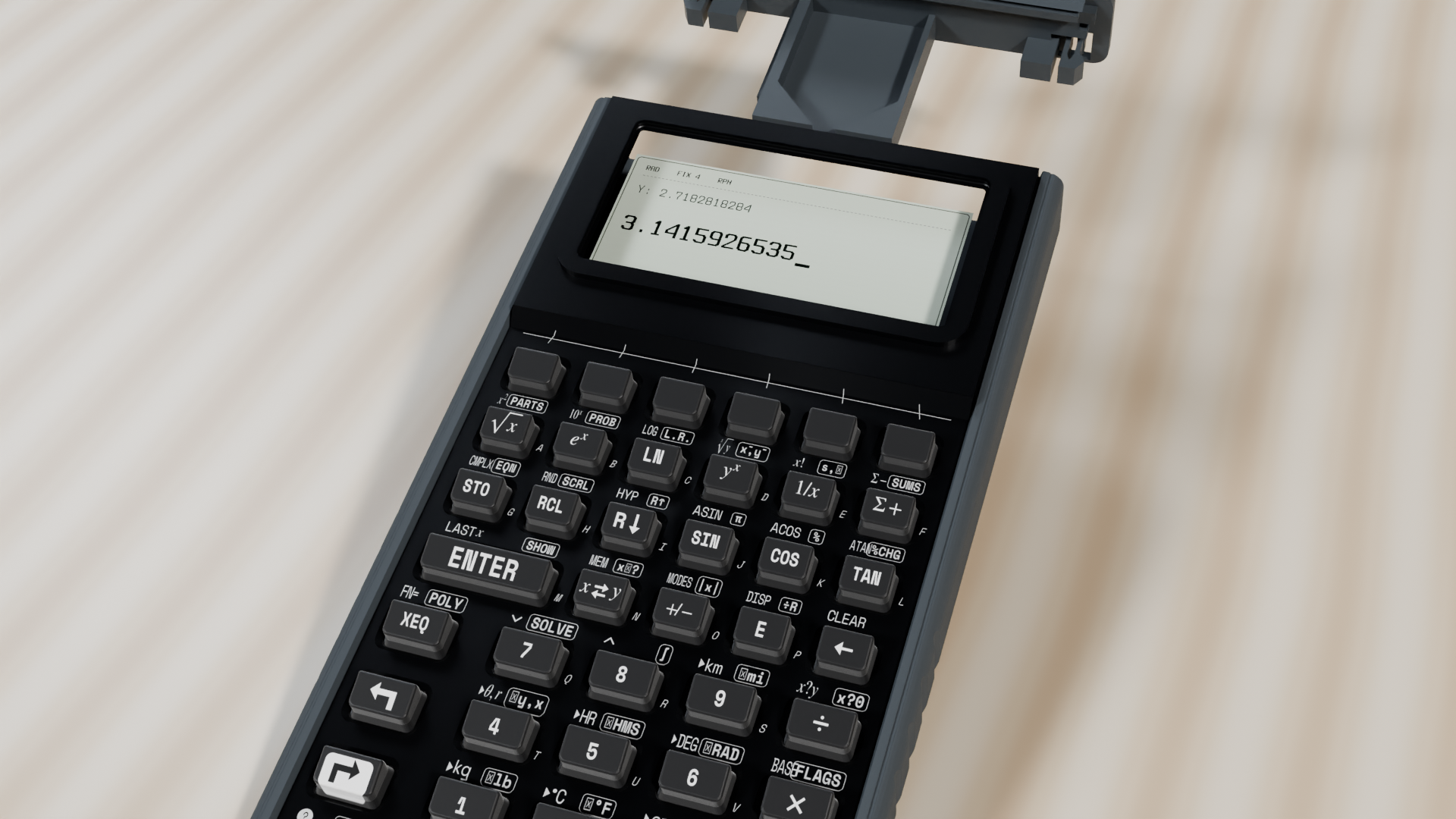
On an electronics or machine-shop workbench, the open-source SC-32 chassis, dovetail service bay (Figure 1.2), and tilted desk cradle are dimensioned to mate with the Gridfinity (\(42\text{ mm} \times 42\text{ mm}\)) modular workshop grid: a \(2 \times 3\) Gridfinity baseplate footprint (\(84\text{ mm} \times 126\text{ mm}\)) seats the instrument at an ergonomic \(18^\circ\) viewing angle beside oscilloscope probes, calipers, and component bins without sliding under one-handed thumb pressure.

---

1.2 Spanning One Hundred Orders of Magnitude: Scientific Notation & Physical Constants

A shirt-pocket instrument meant to replace both a wooden slide rule and a four-function adding machine requires more than four arithmetic keys, because physics, chemistry, and engineering do not live solely in the everyday neighborhood between \(1\) and \(1,000\).

To reason across subatomic and astronomical scales without drowning in leading or trailing zeros, a pocket scientific instrument must separate how accurately a quantity is measured from how large or small that quantity is. When Avogadro's constant (\(N_A \approx 6.022 \times 10^{23}\text{ mol}^{-1}\)) multiplies the elementary charge (\(e \approx 1.602 \times 10^{-19}\text{ C}\)), floating-point scientific notation bridges forty-two orders of magnitude to yield Faraday's macroscopic electrolysis constant \(F = N_A e \approx 96,485.332\text{ C/mol}\).

1.2.1 Separating Shape from Scale: Mantissa and Exponent

In chemistry, a single mole of carbon-12 atoms (\(12\text{ grams}\)) contains Avogadro's number of atoms, \(602,214,076,000,000,000,000,000\). In atomic optics, a red helium-neon laser beam has a vacuum wavelength of \(0.0000006328\text{ meters}\). Writing twenty-three trailing zeros on a chalkboard or counting six leading zeros after a decimal point blurs the eye within seconds, and a single missed zero throws a bridge, orbit, or circuit off by a factor of ten.

To represent quantities spanning sixty orders of magnitude from the subatomic to the cosmological, scientific notation factors every nonzero real number \(x\) into a normalized significand and an integer power of ten:

\[x = m \times 10^n \qquad (1 \le |m| < 10,\; n \in \mathbb{Z}) \tag{Eq. 1.3}\]

The mantissa (or significand) \(m\) contains the meaningful measured digits, or significant figures, normalized so that a single non-zero digit sits to the left of the decimal point (\(6.022\) or \(6.328\)). The mantissa records the shape and precision of the measurement, which is the exact portion that a wooden slide rule displayed along its engraved scale. Paired with the mantissa, the integer exponent \(n\) specifies the order of magnitude, counting how many powers of ten to scale upward for \(n > 0\) or downward for \(n < 0\).

In electrical, mechanical, and optical work, powers of ten that are multiples of three (\(10^{\pm 3k}\)) match the International System of Units (SI) metric prefixes, distinguishing standard scientific notation, where \(1 \le |m| < 10\), from engineering notation, where the exponent \(n\) always locks to a multiple of \(3\). Upward from one thousand, the everyday macro prefixes step by factors of \(10^3\) through kilo (\(10^3\)), mega (\(10^6\)), giga (\(10^9\)), tera (\(10^{12}\)), and peta (\(10^{15}\)) all the way to ronna (\(10^{27}\)) and quetta (\(10^{30}\)); downward from one-thousandth, the micro prefixes step by factors of \(10^{-3}\) through milli (\(10^{-3}\)), micro (\(10^{-6}\)), nano (\(10^{-9}\)), pico (\(10^{-12}\)), and femto (\(10^{-15}\)) down to ronto (\(10^{-27}\)) and quecto (\(10^{-30}\)).

When two numbers in scientific notation are multiplied or divided, their mantissas (\(m_1, m_2\)) multiply or divide while their orders of magnitude (\(n_1, n_2\)) add or subtract:

\[(m_1 \times 10^{n_1}) \times (m_2 \times 10^{n_2}) = (m_1 \times m_2) \times 10^{n_1 + n_2}, \qquad \frac{m_1 \times 10^{n_1}}{m_2 \times 10^{n_2}} = \left(\frac{m_1}{m_2}\right) \times 10^{n_1 - n_2} \tag{Eq. 1.4}\]

A frequent error when entering scientific notation on a calculator is treating \(3 \times 10^8\) as two separate numbers: a number written as \(3 \times 10^8\) is one atomic value, not an arithmetic multiplication problem between \(3\) and \(10^8\). Take the transit time required for a laser pulse traveling at \(c = 3 \times 10^8\text{ m/s}\) to cross a \(d = 1.5\text{ m}\) optical bench (\(t = 1.5 / (3 \times 10^8)\)). If a student using an ordinary calculator enters 1.5 ÷ 3 × 10 ^ 8 as separate arithmetic operations, the calculator divides \(1.5\) by \(3\) first to get \(0.5\) and then multiplies that quotient by \(10^8\). Instead of \(5 \times 10^{-9}\text{ seconds}\) (five nanoseconds), the screen returns \(50,000,000\text{ seconds}\), or nineteen months: an error of sixteen orders of magnitude (\(10^{16}\)).

Scientific instruments prevent this precedence trap by providing a dedicated exponent-entry mechanism that binds the scale factor \(10^n\) to the mantissa inside the numeric entry buffer without issuing an arithmetic multiplication command, so the entire quantity moves through the calculation as a single atomic value. A direct corollary governs pure powers of ten: because the exponent field already represents "\(\times 10^n\)", a pure power of ten like \(10^{-7}\text{ F}\) (\(1 \times 10^{-7}\text{ F}\)) or \(10^6\text{ Hz}\) (\(1 \times 10^6\text{ Hz}\)) carries a leading mantissa of \(1\); pairing a mantissa of \(10\) with an exponent of \(6\) produces \(10 \times 10^6 = 10^7\), a tenfold order-of-magnitude error.

How a number is formatted on the screen—whether rounded to fixed decimal places, normalized in scientific notation, or grouped in engineering powers of three—never truncates or rounds the underlying value in memory, where every stack register (\(X, Y, Z, T\)) and named variable (\(A\dots Z\)) retains full IEEE 754 double precision (\(53\text{ bits}\) of binary significand, or roughly \(15\) to \(17\) decimal digits). In laboratory calibration, however, an engineer working with two or three visible decimals often needs to inspect the unrounded internal mantissa to verify whether two nearly equal bridge measurements differ in the twelfth decimal place. A momentary full-mantissa inspection view solves this by revealing all internal digits of Register \(X\) on demand without altering the active display format.

Alongside the BIPM powers of ten, international metrology standards fix the conversion factors between customary Imperial measurements and SI units without experimental uncertainty: exact inch-to-centimeter length (\(1\text{ in} \equiv 2.54\text{ cm}\) and \(1\text{ ft} \equiv 0.3048\text{ m}\)), statute and nautical miles (\(1\text{ mi} \approx 1.609\text{ km}\) and \(1\text{ nmi} \equiv 1,852\text{ m}\)), avoirdupois mass (\(1\text{ lb} \approx 0.454\text{ kg}\)), U.S. liquid volume (\(1\text{ gal} \equiv 231\text{ in}^3 \approx 3.785\text{ L}\)), standard atmospheric pressure (\(1\text{ atm} \equiv 101,325\text{ Pa}\)), thermochemical energy (\(1\text{ cal}_{\text{th}} \equiv 4.184\text{ J}\)), affine Fahrenheit-to-Celsius temperature (\(T_{\text{C}} = (T_{\text{F}} - 32) \times \frac{5}{9}\)), and sexagesimal-to-decimal time or angle (\(H + \frac{M}{60} + \frac{S}{3600}\)). Because a square inch equals \((2.54\text{ cm})^2 \approx 6.452\text{ cm}^2\) and a cubic inch equals \((2.54\text{ cm})^3 \approx 16.387\text{ cm}^3\), scaling a cross-sectional area twice or an engine displacement three times in succession by the linear factor \(2.54\) converts \(\text{in}^2 \leftrightarrow \text{cm}^2\) and \(\text{in}^3 \leftrightarrow \text{cm}^3\) without memorizing separate area or volume constants.

1.2.2 Why Every Digital Watch Vibrates 32,768 Times a Second

Beyond representing microscopic and astronomical numbers, a pocket scientific instrument must also measure physical time without the temperature drift of a mechanical balance wheel. That timebase comes from piezoelectricity inside crystalline \(\alpha\)-quartz (\(\text{SiO}_2\), silicon dioxide). When a quartz crystal is compressed or sheared mechanically, the positive silicon ions and negative oxygen ions in its non-centrosymmetric trigonal lattice shift slightly apart and generate an electrical potential across its faces; under the converse piezoelectric effect, applying an alternating voltage across metal electrodes plated onto the quartz wafer causes the crystal to expand, contract, and flex like a microscopic tuning fork.

Because a single crystal of quartz is an almost perfectly elastic atomic lattice with near-zero internal friction in a vacuum, a laser-trimmed quartz tuning fork just four millimeters long rings thousands of times longer than a steel tuning fork. The specification sheet for almost any digital wristwatch, spacecraft timer, or the real-time clock inside the SC-32 lists a characteristic vibration frequency:

\[f_{\text{RTC}} = 32,768\text{ Hz} \tag{Eq. 1.5}\]

Electrical engineers chose \(32,768\) vibrations per second rather than a round decimal frequency such as \(10,000\text{ Hz}\) or \(50,000\text{ Hz}\) for a binary reason. Because frequency \(f\) (in hertz, cycles per second) and period \(T\) (in seconds per cycle) are exact reciprocals (\(T = 1/f\)), each single swing of a \(32,768\text{ Hz}\) quartz tuning fork takes \(T = 1 / 32,768\text{ Hz} \approx 30.518\text{ microseconds}\). In binary CMOS electronics, the simplest frequency-dividing element is a toggle flip-flop, a bistable sequential circuit that changes state on every rising (or falling) clock edge and divides the incoming frequency in half (\(\div 2\)). Chaining fifteen divide-by-two flip-flops in series halves the frequency at every stage:

\[32,768 \xrightarrow{\div 2} 16,384 \xrightarrow{\div 2} 8,192 \xrightarrow{\div 2} 4,096 \xrightarrow{\div 2} \dots \xrightarrow{\div 2} 4 \xrightarrow{\div 2} 2 \xrightarrow{\div 2} 1\text{ pulse per second} \tag{Eq. 1.6}\]

Because \(2^{15} = 32,768\), fifteen ultra-low-power halving stages reduce \(32,768\text{ Hz}\) down to \(1\text{ Hz}\) without a single decimal comparator. The choice of \(2^{15} = 32,768\text{ Hz}\) over \(2^{14} = 16,384\text{ Hz}\) follows from the upper limit of human hearing near \(20,000\text{ Hz}\): a \(16,384\text{ Hz}\) crystal would emit a faint, high-pitched whine near the ear, while \(32,768\text{ Hz}\) is the first ultrasonic, inaudible power of two.

While a \(32,768\text{ Hz}\) tuning-fork crystal keeps human calendar time during deep sleep on nanoamperes of current, waking the processor to compute a Romberg definite integral or a closed-form cubic root sweep in milliseconds requires a much faster heartbeat: a \(12\text{ MHz}\) (\(1.2 \times 10^7\text{ Hz}\)) Pierce quartz crystal oscillator, whose period is \(T = 1 / (1.2 \times 10^7\text{ Hz}) \approx 83.333\text{ nanoseconds}\).

Just as adding a small calibration weight to a pendulum bob fine-tunes its oscillation rate, a Pierce quartz wafer requires a specific effective load capacitance \(C_L\) across its terminals to resonate at its nominal factory frequency. On the circuit board, two symmetric ceramic capacitors (\(C_1 = C_2 = C\)) sit at the input and output pins of the crystal, wired in series with each other through the ground plane to form a series branch capacitance \(C_{\text{series}}\), while the copper PCB traces and amplifier pins contribute an unavoidable parallel stray capacitance \(C_{\text{stray}}\). Because two equal capacitors in series trap the same charge across twice the dielectric gap, their combined series capacitance is \(C/2\), which adds in parallel with \(C_{\text{stray}}\) to supply the crystal's total load capacitance \(C_L\):

\[C_{\text{series}} = C_1 \parallel C_2 = \frac{C_1 C_2}{C_1 + C_2} = \frac{C^2}{2C} = \frac{C}{2}, \qquad C_L = \frac{C}{2} + C_{\text{stray}} \implies C = 2(C_L - C_{\text{stray}}) \tag{Eq. 1.7}\]

Subtracting the board's unavoidable stray capacitance \(C_{\text{stray}}\) from the crystal's target load \(C_L\) leaves the net series capacitance that the external network must provide, and doubling that difference compensates for the series halving across the two symmetric pins. For the \(12\text{ MHz}\) Pierce quartz crystal to resonate at its calibrated factory frequency with \(C_L = 18\text{ pF}\) and PCB stray capacitance \(C_{\text{stray}} = 3.5\text{ pF}\), the external network must supply \(18 - 3.5 = 14.5\text{ pF}\) in series, specifying \(C = 2(14.5) = \mathbf{29}\text{ pF}\) per external load capacitor.

Temperature changes also tug on the elastic stiffness of quartz, shifting an oscillator's live frequency away from its calibrated nominal frequency \(f_0\) by a fractional frequency drift \(\Delta f / f_0\) as the operating temperature \(T\) departs from the reference turnover or inflection temperature \(T_0 = 25^\circ\text{C}\). How the crystal responds to temperature depends on the angle at which the wafer is sawed from the raw quartz boule. A miniature \(32,768\text{ Hz}\) tuning-fork real-time clock crystal is cut so its frequency peaks at \(T_0 = 25^\circ\text{C}\) and bends downward with parabolic curvature constant \(k_2 = 0.035\text{ ppm/K}^2\) (\(0.035 \times 10^{-6}\text{ K}^{-2}\)). By contrast, slicing a high-frequency quartz boule along a plane inclined at \(35^\circ 15'\) to the optical \(Z\)-axis—the AT-cut orientation—cancels both the linear and quadratic temperature slopes at the inflection temperature \(T_0 = 25^\circ\text{C}\), leaving only a gentle third-order cubic curvature constant \(k\):

\[\frac{\Delta f}{f_0} = -k_2(T - T_0)^2 \quad \text{(tuning-fork cut)}, \qquad \frac{\Delta f}{f_0} = k(T - T_0)^3 \quad \text{(AT-cut)} \tag{Eq. 1.8}\]

Squaring the temperature departure \((T - T_0)\) in the tuning-fork response makes \((T - T_0)^2\) positive on both sides of \(25^\circ\text{C}\), so the leading minus sign causes a wristwatch or real-time clock crystal to slow down and lose time whether it is warmed above \(25^\circ\text{C}\) or chilled below \(25^\circ\text{C}\). The AT-cut's cubic dependence \((T - T_0)^3\), by contrast, creates a wide, flat plateau around room temperature while preserving the sign of \((T - T_0)\), drifting slightly fast in extreme heat and slightly slow in deep cold. When that \(12\text{ MHz}\) AT-cut wafer cools from \(T_0 = 25^\circ\text{C}\) to a \(T = -15^\circ\text{C}\) winter field site (\(\Delta T = T - T_0 = -40\text{ K}\), cubic coefficient \(k = 0.035 \times 10^{-9}\text{ K}^{-3}\)), the cubic excursion \((-40\text{ K})^3 = -64,000\text{ K}^3\) produces a fractional shift of \(\Delta f / f_0 = \mathbf{-2.24 \times 10^{-6}}\) (\(-2.24\text{ ppm}\)), or \(\Delta f = \mathbf{-26.88\text{ Hz}}\) on the \(12\text{ MHz}\) carrier (\(\approx -0.194\text{ s/day}\)).

Beside the processor's power pins sit ceramic bypass capacitors of capacitance \(C\) that shunt high-frequency transistor switching noise to ground. Every surface-mount capacitor has metal end-caps and internal plates that form a small current loop with equivalent series inductance \(L_{\text{ESL}}\), whose inductive reactance \(X_L = 2\pi f L_{\text{ESL}}\) grows linearly with frequency \(f\) while capacitive reactance \(X_C = \frac{1}{2\pi f C}\) drops hyperbolically. At the exact crossover frequency where \(X_C = X_L\), the opposing electric and magnetic reactances cancel to zero and the capacitor reaches its self-resonant frequency \(f_{\text{SRF}}\):

\[f_{\text{SRF}} = \frac{1}{2\pi \sqrt{L_{\text{ESL}} C}} \tag{Eq. 1.9}\]

Shrinking either the package loop inductance \(L_{\text{ESL}}\) or the capacitance \(C\) shortens the electromagnetic sloshing time \(\sqrt{L_{\text{ESL}}C}\) and pushes the self-resonant crossover \(f_{\text{SRF}}\) to a higher frequency, above which parasitic inductance dominates and the component begins behaving like an inductor rather than a capacitor. For a \(C = 100\text{ nF}\) (\(10^{-7}\text{ F}\)) decoupling capacitor with package inductance \(L_{\text{ESL}} = 0.85\text{ nH}\) (\(8.5 \times 10^{-10}\text{ H}\)), the characteristic time \(\sqrt{L_{\text{ESL}}C} \approx 9.22\text{ ns}\) sets the self-resonant crossover at \(f_{\text{SRF}} \approx \mathbf{17.263\text{ MHz}}\).

1.2.3 Fixing the Constants of Nature: The 2019 SI Redefinition

Quantum mechanics, relativity, and statistical physics regularly combine quantities separated by more than fifty orders of magnitude inside a single equation. At the subatomic boundary sit Planck's action quantum \(h \sim 10^{-34}\text{ J}\cdot\text{s}\) and the electron rest mass \(m_e \sim 10^{-30}\text{ kg}\); at the relativistic horizon sit the squared vacuum speed of light \(c^2 \sim 10^{17}\text{ m}^2/\text{s}^2\) and Avogadro's molar count \(N_A \sim 10^{23}\text{ mol}^{-1}\). On any fixed-point mechanical calculator or integer register, multiplying or dividing across fifty powers of ten underflows to zero or overflows the carriage. Only by separating the 53-bit IEEE 754 significand from its signed base-10 exponent can a pocket instrument hold Planck's constant and the squared speed of light side by side without losing a single significant figure.

Under the 2019 SI Redefinition, the defining constants of the system (\(c = 299,792,458\text{ m/s}\), Planck's constant \(h \approx 6.626 \times 10^{-34}\text{ J}\cdot\text{s}\), the elementary charge \(e \approx 1.602 \times 10^{-19}\text{ C}\), Boltzmann's constant \(k_B \approx 1.381 \times 10^{-23}\text{ J/K}\), and Avogadro's constant \(N_A \approx 6.022 \times 10^{23}\text{ mol}^{-1}\)) are fixed as exact numerical invariants with zero measurement uncertainty, which in turn fixes exact values for derived combinations, including the molar gas constant (\(R = N_A k_B \approx 8.314\text{ J/(mol}\cdot\text{K)}\)) and the Stefan–Boltzmann constant (\(\sigma = \frac{2\pi^5 k_B^4}{15 c^2 h^3} \approx 5.67 \times 10^{-8}\text{ W/(m}^2\cdot\text{K}^4)\)). Alongside these invariants stand the experimentally measured constants—the Newtonian gravitational constant (\(G \approx 6.674 \times 10^{-11}\text{ N}\cdot\text{m}^2/\text{kg}^2\)), vacuum permittivity (\(\varepsilon_0 \approx 8.854 \times 10^{-12}\text{ F/m}\)), and vacuum permeability (\(\mu_0 \approx 1.257 \times 10^{-6}\text{ N/A}^2\))—and the fundamental mathematical constants \(\pi \approx 3.142\) (π) and the natural base \(e \approx 2.718\).

Across optics, atomic physics, relativistic mechanics, and nuclear decay, these invariants bridge the wave and particle worlds. In quantum optics, a beam of light of vacuum wavelength \(\lambda\) and oscillation frequency \(\nu = c/\lambda\) delivers its energy not as a continuous wash, but in discrete quanta of photon energy \(E_{\text{photon}} = h\nu\). Conversely, Louis de Broglie showed that any massive particle of mass \(m\) traveling at velocity \(v\)—carrying linear momentum \(p = mv\)—propagates with an intrinsic matter-wave wavelength \(\lambda_{\text{deB}}\):

\[E_{\text{photon}} = \frac{h c}{\lambda}, \qquad \lambda_{\text{deB}} = \frac{h}{m v} \tag{Eq. 1.10}\]

Halving the optical wavelength \(\lambda\) packs twice as much energy into each quantum of light through the universal scale factor \(hc \approx 1.986 \times 10^{-25}\text{ J}\cdot\text{m}\). At the green solar peak (\(\lambda = 500 \times 10^{-9}\text{ m}\)), a single photon carries \(E_{\text{photon}} \approx 3.973 \times 10^{-19}\text{ J}\), or \(\approx \mathbf{2.48\text{ eV}}\) after dividing by the electron-volt conversion factor \(e \approx 1.602 \times 10^{-19}\text{ J/eV}\)—which is why one short-wavelength ultraviolet or X-ray photon can eject a bound inner-shell electron that no flood of long-wavelength infrared photons can dislodge.

Accelerating a massive particle to higher momentum \(p = mv\) similarly compresses its matter wave \(\lambda_{\text{deB}} = h/(mv)\) into a tighter spatial period (with the Compton wavelength \(\lambda_C = h / (m_e c) \approx 2.426 \times 10^{-12}\text{ m}\) marking the scale where photon momentum equals \(m_e c\)). An electron (\(m_e \approx 9.109 \times 10^{-31}\text{ kg}\)) accelerated down an electron-microscope column to \(v = 2 \times 10^6\text{ m/s}\) has specific quantum diffusivity \(h/m_e \approx 7.274 \times 10^{-4}\text{ m}^2/\text{s}\) and a de Broglie wavelength of \(\lambda_{\text{deB}} \approx 3.637 \times 10^{-10}\text{ m}\) (\(\approx \mathbf{0.364\text{ nm}}\)), fine enough to resolve individual crystal lattices.

Inside an atom, those electron matter waves wrap around the nucleus as standing waves, restricting bound electrons to discrete principal quantum shells indexed by integers \(n_1 < n_2\). Because the binding energy of the \(n\)-th Bohr shell scales inversely with the square of its shell number (\(1/n^2\)), an electron dropping from an outer shell \(n_2\) down to an inner shell \(n_1\) radiates a photon whose spectral wavenumber \(1/\lambda\) (waves per meter) is governed by the Rydberg constant \(R_\infty \approx 1.097 \times 10^7\text{ m}^{-1}\):

\[\frac{1}{\lambda} = R_{\infty}\left(\frac{1}{n_1^2} - \frac{1}{n_2^2}\right) \tag{Eq. 1.11}\]

Each quantum jump from an outer orbit \(n_2\) down to an inner orbit \(n_1\) releases a fraction \(\frac{1}{n_1^2} - \frac{1}{n_2^2}\) of hydrogen's ground-state ionization energy, and scaling that dimensionless step by \(R_\infty\) fixes the radiated wavenumber \(1/\lambda\). For the solar Balmer \(H_\alpha\) transition (\(n_2 = 3 \to n_1 = 2\), where \(1/2^2 - 1/3^2 = 5/36 \approx 0.139\)), the wavenumber \(\approx 1.524 \times 10^6\text{ m}^{-1}\) evaluated in the infinite-nuclear-mass Rydberg limit (\(R_\infty \approx 10,973,731.568\text{ m}^{-1}\)) inverts to the deep-red vacuum wavelength \(\lambda \approx \mathbf{656.112\text{ nm}}\) (or \(\approx 656.335\text{ nm}\) from the three-decimal approximation \(1.097 \times 10^7\text{ m}^{-1}\)).

At the opposite end of the velocity and energy spectrum, relativistic kinematics unifies a particle's rest mass \(m\), velocity \(v\), momentum \(p\), and total energy \(E\) through the spacetime invariant \(E^2 = (pc)^2 + (mc^2)^2\). For a mass at rest (\(p = 0\)), total energy reduces to the rest energy \(E = mc^2\); for a particle accelerated to a large fraction \(\beta = v/c\) of the speed of light, its classical momentum \(mv\) is amplified by the dimensionless Lorentz factor \(\gamma = 1/\sqrt{1 - (v/c)^2}\):

\[E = m c^2, \qquad p = \gamma m v = \frac{m v}{\sqrt{1 - (v/c)^2}} \tag{Eq. 1.12}\]

Because the squared speed of light \(c^2 \approx 8.988 \times 10^{16}\text{ J/kg}\) multiplies rest mass by nearly ninety quadrillion joules per kilogram, a nuclear fission or fusion reaction that converts a \(1\text{ gram}\) (\(10^{-3}\text{ kg}\)) mass defect into kinetic and radiative energy releases \(E = mc^2 \approx 8.988 \times 10^{13}\text{ J}\) (\(\approx \mathbf{89.876\text{ TJ}}\)). Meanwhile, as a particle's speed \(v\) approaches \(c\), the ratio \(v/c\) nears unity and the radical \(\sqrt{1-(v/c)^2}\) shrinks toward zero, driving the Lorentz factor \(\gamma\) and momentum \(p = \gamma mv\) upward without bound so no finite force can accelerate a massive particle past light speed. Accelerating a synchrotron proton (\(m_p \approx 1.673 \times 10^{-27}\text{ kg}\)) to \(v = 0.85c \approx 2.548 \times 10^8\text{ m/s}\) (\(\beta = 0.85\)) contracts \(\sqrt{1 - 0.85^2}\) to \(\approx 0.527\) (\(\gamma \approx 1.898\)), raising its effective inertia to \(\gamma m_p \approx 3.175 \times 10^{-27}\text{ kg}\) and its relativistic momentum to \(p = \gamma m_p v \approx \mathbf{8.091 \times 10^{-19}\text{ kg}\cdot\text{m/s}}\)—which fixes the magnetic dipole rigidity \(B\rho = p/e\), the product of magnetic field strength \(B\) and bending radius \(\rho\) needed to guide a unit charge \(e\) around the storage ring.

Inside unstable atomic nuclei, random quantum tunneling triggers radioactive decay at a constant fractional decay rate \(\lambda_{\text{dec}} = \ln(2)/t_{1/2}\) (distinct from optical wavelength \(\lambda\)), where the half-life \(t_{1/2}\) is the time required for half of an initial population of \(N_0\) nuclei (or initial radioactive activity \(A_0 = \lambda_{\text{dec}} N_0\)) to transform into daughter nuclei. Over an elapsed time \(t\), the surviving population \(N(t)\)—and its proportional activity \(A(t)\)—follows continuous exponential or base-\(1/2\) decay:

\[N(t) = N_0 e^{-\lambda_{\text{dec}} t} = N_0 \left(\frac{1}{2}\right)^{t / t_{1/2}}, \qquad A(t) = A_0 \left(\frac{1}{2}\right)^{t / t_{1/2}} \tag{Eq. 1.13}\]

Every elapsed half-life increments the dimensionless ratio \(t / t_{1/2}\) by \(1\) and cuts the surviving population \(N(t)\) and activity \(A(t)\) in half. After \(t = 15\text{ yr}\), a Cobalt-60 beta-decay teletherapy source of initial activity \(A_0 = 10,000\text{ Bq}\) and half-life \(t_{1/2} = 5.27\text{ yr}\) has passed through \(t/t_{1/2} = 15/5.27 \approx 2.846\) half-lives, retaining \(A(15\text{ yr}) = 10,000 \times (1/2)^{15/5.27} \approx \mathbf{1,390.524\text{ Bq}}\).

---

1.3 Reflecting the Sun and Nursing a Coin Cell

Whereas early red-LED pocket calculators drained their rechargeable batteries in forty-five minutes and washed out in direct sunlight, a transflective instrument operates for months or years on a single lithium coin cell. Three keypad mechanisms on the SC-32 link unit conversions, scientific notation, and display formatting to the four-register stack (T, Z, Y, X):

1. In-Place SI \(\leftrightarrow\) Imperial Unit Conversions: Ten physical unit conversions sit on the lower keypad—Left Shift [↰] always converts into Metric ([↰] [▸kg] on 1, [↰] [▸°C] on 2, [↰] [▸cm] on 3, [↰] [▸l] on -, [↰] [▸km] on 9, and [↰] [▸DEG] on 6), while Right Shift [↱] always converts into Imperial/Radians ([↱] [▸lb] on 1, [↱] [▸°F] on 2, [↱] [▸in] on 3, [↱] [▸gal] on -, [↱] [▸mi] on 9, and [↱] [▸RAD] on 6). Every conversion transforms Register \(X\) in place and arms automatic stack lift so the next number typed pushes the converted figure up into Registers \(Y, Z,\) and \(T\). Applying a linear conversion twice in succession ([↰] [▸cm] [↰] [▸cm] or [↱] [▸in] [↱] [▸in]) converts cross-sectional area (\(\text{in}^2 \leftrightarrow \text{cm}^2\)), and applying it three times ([↰] [▸cm] [↰] [▸cm] [↰] [▸cm]) converts cubic displacement (\(\text{in}^3 \leftrightarrow \text{cm}^3\)) in place.
2. Scientific Exponent Entry ([E]), Euclidean Remainder ([↱] [÷R]), Display Formatting ([↰] [DISP]), & Full-Mantissa Inspection ([↱] [SHOW]): The [E] key binds base-10 exponents inside the entry buffer (8 [E] 6 enters \(8 \times 10^6\), and 1 [E] 7 [+/-] enters \(10^{-7}\)), while right-shifted [↱] [÷R] on [E] divides Register \(Y\) by Register \(X\) into an integer quotient in \(X\) and remainder in \(Y\). Left-shifted [↰] [DISP] on [E] populates the softkey strip with: $\(\mathtt{[FIX]} \quad \mathtt{[SCI]} \quad \mathtt{[ENG]} \quad \mathtt{[ALL]}\)$ By default, ALL displays numbers in clean general form with trailing zeros suppressed; tapping FIX, SCI, or ENG prompts FIX _ (or SCI _, ENG _) for a digit 0–9 to format the LCD without altering the full 64-bit value in the registers, while pressing [↱] [SHOW] (right-shifted on [ENTER]) reveals the full unrounded 53-bit internal significand of Register \(X\) (or both parts of a complex number when preceded by [↰] [CMPLX]) without changing the active [↰] [DISP] mode.
3. Graduated Clearing ([<-], [C], [↰] [CLEAR]) & On-Device Guidance ([↰] [?]): Unshifted [<-] backspaces live digit entry (or zeroes Register \(X\) once a calculation is complete). Left-shifted [↰] [CLEAR] on [<-] opens \(\mathtt{[CLEQN]} \;\; \mathtt{[CLVARS]} \;\; \mathtt{[CLALL]} \;\; \mathtt{[CLSTAT]} \;\; \mathtt{[CLREGS]} \;\; \mathtt{[CLSTK]}\) to clear equations, variables, statistical sums, storage registers, or the four-level stack independently, and left-shifted [↰] [?] on [C] launches the built-in interactive tutorial on the LCD.

1.3.1 Pre-Flight Manifests and Sunlight-Reflective Glass

On a hot ramp (\(86^\circ\text{F}\)), a bush pilot who loads \(52\text{ US gallons}\) of 100LL avgas (at the standard FAA nominal weight of \(6\text{ lb/gal}\)) can record the metric fuel mass, metric fuel volume, Celsius outside air temperature, and a \(25.4\text{ cm}\) propeller-tip ground clearance in inches across the four stack lines without clearing a single intermediate result. Multiplying \(52 \times 6 = 312\text{ lb}\) and converting pounds to kilograms transforms Register \(X\) in place to \(\approx \mathbf{141.521\text{ kg}}\) while arming stack lift; keying \(52\) and converting gallons to liters lifts the fuel mass into Register \(Y\) and places \(\approx \mathbf{196.841\text{ L}}\) in Register \(X\); keying \(86\) and converting Fahrenheit to Celsius lifts both fuel figures upward and places \(\mathbf{30^\circ\text{C}}\) in Register \(X\); and keying \(25.4\) and converting centimeters to inches lifts all three prior figures and places \(\mathbf{10\text{ in}}\) in Register \(X\), so all four pre-flight numbers (\(\approx 141.521\text{ kg}\) in \(T\), \(\approx 196.841\text{ L}\) in \(Z\), \(30^\circ\text{C}\) in \(Y\), and \(10\text{ in}\) in \(X\)) remain visible together on the display.

The transflective liquid-crystal display (LCD) that renders those four registers in direct noon sunlight harvests ambient light instead of fighting it with high-power emission. Whereas an emissive smartphone screen must overcome \(100,000\text{-lux}\) sky irradiance with hundreds of milliwatts of backlight power, a transflective panel reflects incident sunlight off a brushed metallic backing behind twisted-nematic liquid-crystal molecules, sharpening in brighter sunlight while drawing a fraction of a milliwatt. Streaming a full \(132 \times 65\) frame buffer (\(N_{\text{cmd}} = 9\) command bytes plus \(N_{\text{col}} = 1,056\) pixel-column bytes, or \(1,065\text{ bytes} = 8,520\text{ bits}\)) over an \(f_{\text{SPI}} = 8 \times 10^6\text{ bits/s}\) serial bus takes just \(8,520 / (8 \times 10^6) = \mathbf{1.065\text{ ms}}\), allowing the display bus to sleep for \(\approx 99.89\%\) of every second. And because liquid-crystal molecules stiffen as ambient temperature \(T\) drops and their rotational viscosity \(\gamma_1(T)\) thickens like cold honey, a fixed drive voltage would leave outdoor winter digits sluggish and faded. To keep contrast crisp across all weather, the on-chip charge pump adjusts the live LCD bias voltage \(V(T)\) around its room-temperature reference voltage \(V_0 = 9\text{ V}\) (at \(T_0 = 25^\circ\text{C}\)) using a negative linear temperature slope \(\frac{dV}{dT} = -12.5\text{ mV/}^\circ\text{C}\) (\(\approx -0.013\text{ V/}^\circ\text{C}\)):

\[V(T) = V_0 + \frac{dV}{dT}(T - T_0) \tag{Eq. 1.14}\]

Because both the slope \(\frac{dV}{dT}\) and the cold temperature excursion \((T - T_0)\) are negative below \(25^\circ\text{C}\), their product \(\frac{dV}{dT}(T - T_0)\) is positive, automatically boosting the electric field when the fluid is stiff and relaxing it when the fluid is warm. In freezing air (\(T = 0^\circ\text{C}\), \(\Delta T = T - T_0 = -25^\circ\text{C}\)), that linear offset raises the LCD bias rail by \((-12.5\text{ mV/}^\circ\text{C})(-25^\circ\text{C}) = +312.5\text{ mV} \approx +0.313\text{ V}\) to \(V(0^\circ\text{C}) \approx \mathbf{9.313}\text{ V}\) so numerals neither ghost nor fade outdoors.

1.3.2 Laser-Foamed Legends and the Thévenin Coin Cell

Around that reflective glass, the dark matte polymer shell is compounded with carbon-black pigment so stray sunlight and near-infrared radiation cannot penetrate the walls and scatter across the optical cavity. When a beam of incident intensity \(I_0\) enters the plastic, radiation attenuates exponentially with depth \(z\) because each uniform layer absorbs the same fraction of the photons reaching it: if the first layer absorbs half of the incoming flux, the next layer of equal thickness absorbs half of the remainder, reducing the transmitted intensity \(I(z)\) to one-quarter and then one-eighth. Integrating the differential loss \(dI/dz = -\alpha I\) across the material's linear absorption coefficient \(\alpha\) yields the Beer–Lambert attenuation law for \(I(z)\), which inverts via the natural logarithm to give the penetration depth \(z\) where intensity falls to a fraction \(I/I_0\). During manufacturing, this shallow optical skin is exploited to mark permanent, wear-proof keycap legends without ink: a Q-switched fiber laser operating at average power \(P_{\text{avg}}\) chops its beam at pulse repetition frequency \(f_{\text{rep}}\) into discrete packets of pulse energy \(E_{\text{pulse}}\), compresses each packet into a brief pulse duration \(\tau\) to reach an intense peak power \(P_{\text{peak}}\), and focuses that energy onto a circular spot of radius \(r\) (area \(\pi r^2\)) to deliver a foaming surface fluence \(F\) (energy per unit area):

\[I(z) = I_0 e^{-\alpha z} \implies z = -\frac{\ln(I/I_0)}{\alpha}, \qquad E_{\text{pulse}} = \frac{P_{\text{avg}}}{f_{\text{rep}}}, \qquad P_{\text{peak}} = \frac{E_{\text{pulse}}}{\tau}, \qquad F = \frac{E_{\text{pulse}}}{\pi r^2} \tag{Eq. 1.15}\]

High pigment absorption \(\alpha\) confines the transmitted fraction \(I/I_0 < 1\) (where \(-\ln(I/I_0) > 0\)) to a shallow surface skin \(z\), preventing heat from penetrating and warping the keycap core. Although each pulse carries only a tiny energy packet \(E_{\text{pulse}} = P_{\text{avg}}/f_{\text{rep}}\), releasing that packet across a nanosecond Q-switched window \(\tau\) drives instantaneous peak power \(P_{\text{peak}} = E_{\text{pulse}}/\tau\) to hundreds of watts, and focusing the beam onto a microscopic disk of area \(\pi r^2\) reaches the threshold fluence \(F\) needed to nucleate permanent micro-foam legends.

For a \(90\%\) near-infrared attenuation target (\(I/I_0 = 0.1\)) in a pigment-loaded polymer of absorption coefficient \(\alpha = 450\text{ cm}^{-1}\), the Beer–Lambert ratio \(-\ln(0.1)/450 \approx 5.117 \times 10^{-3}\text{ cm}\) confines absorption to the top \(z \approx \mathbf{51.169}\,\mu\text{m}\) skin. Chopping \(P_{\text{avg}} = 1.2\text{ W}\) of average laser power at \(f_{\text{rep}} = 35,000\text{ Hz}\) produces \(E_{\text{pulse}} = 1.2 / 35,000 \approx 3.43 \times 10^{-5}\text{ J}\) (\(\approx 34.286\,\mu\text{J}\)) per packet, and compressing that packet into \(\tau = 10^{-7}\text{ s}\) (\(100\text{ ns}\)) amplifies peak power nearly 300-fold to \(P_{\text{peak}} \approx \mathbf{342.857}\text{ W}\). Across a focal spot of radius \(r = 0.00225\text{ cm}\), the foaming fluence \(F = E_{\text{pulse}} / (\pi r^2)\) evaluates as a two-branch quotient: once \(z \approx 51.169\,\mu\text{m}\) is complete in Register \(X\), starting \(E_{\text{pulse}} = 1.2 / 35,000 \approx 3.43 \times 10^{-5}\text{ J}\) lifts \(z\) into the upper registers, and \(E_{\text{pulse}}\) waits in Register \(Y\) while the spot area \(A = \pi r^2 \approx 1.59 \times 10^{-5}\text{ cm}^2\) forms in Register \(X\) before division yields \(F \approx \mathbf{2.156\text{ J/cm}^2}\) inside that \(51\,\mu\text{m}\) skin.

That same two-branch pattern, where a completed numerator waits in Register \(Z\) while a denominator forms across Registers \(Y\) and \(X\), governs the electrochemical telemetry of the CR2032 lithium-manganese-dioxide (\(\text{Li/MnO}_2\)) coin cell (\(3\text{ V}\) nominal open-circuit electromotive force \(\mathcal{E}\), \(225\text{ mAh}\) capacity) and the copper printed-circuit-board traces that distribute its power. No real battery is an ideal voltage source: as load current \(I\) flows through the cell's finite ion-diffusion pathways, modeled as an equivalent series internal resistance \(R_{\text{int}}\), some electrical potential is lost inside the cell before reaching the external contacts, leaving a reduced terminal voltage \(V_{\text{term}}(I)\). Similarly, when that current travels along a rectangular copper PCB trace of electrical resistivity \(\rho\), length \(L\), width \(w\), and thickness \(t\), electron scattering imposes an ohmic trace resistance \(R\):

\[V_{\text{term}}(I) = \mathcal{E} - I R_{\text{int}}, \qquad R_{\text{int}} = \frac{V_1 - V_2}{I_2 - I_1}, \qquad R = \frac{\rho L}{w t} \tag{Eq. 1.16}\]

Internal electrolyte resistance drops the cell's terminal voltage by \(I R_{\text{int}}\) before power ever reaches the contacts, causing \(V_{\text{term}}\) to sag linearly with current draw \(I\). Comparing the voltage droop \(V_1 - V_2\) against the current step \(I_2 - I_1\) between two live operating states isolates \(R_{\text{int}}\) directly without disconnecting the cell to measure \(\mathcal{E}\), while widening a copper PCB trace of cross-sectional area \(wt\) reduces its series path resistance \(R = \rho L/(wt)\) downstream.

Across an idle display refresh (\(I_1 = 0.0048\text{ A}\), \(V_1 = 2.94\text{ V}\)) and a high-current numerical solver burst (\(I_2 = 0.0182\text{ A}\), \(V_2 = 2.685\text{ V}\)), the voltage droop \(\Delta V = 2.94 - 2.685 = 0.255\text{ V}\) waits in Register \(Z\) while the current step \(\Delta I = 0.0182 - 0.0048 = 0.0134\text{ A}\) forms across Registers \(Y\) and \(X\), dividing to a dynamic internal resistance of \(R_{\text{int}} \approx \mathbf{19.03\,\Omega}\) and internal cell heating \(I_2^2 R_{\text{int}} \approx \mathbf{6.303\text{ mW}}\). By comparison, the 1-oz copper PCB power trace delivering that current (\(\rho = 1.68 \times 10^{-5}\,\Omega\cdot\text{mm}\), length \(L = 45\text{ mm}\), width \(w = 0.25\text{ mm}\), thickness \(t = 0.035\text{ mm}\)) has an ohmic resistance of \(R = \rho L/(wt) \approx 0.086\,\Omega\) and dissipates \(I_2^2 R \approx \mathbf{28.619\,\mu\text{W}}\).

Over an accelerated 24-hour factory stress schedule—\(0.5\text{ h}\) of solver bursts at \(18.2\text{ mA}\) (\(9.1\text{ mAh}\)), \(1.5\text{ h}\) of key entry at \(4.8\text{ mA}\) (\(7.2\text{ mAh}\)), \(2\text{ h}\) of active standby at \(0.85\text{ mA}\) (\(1.7\text{ mAh}\)), and \(20\text{ h}\) of deep sleep at \(0.0118\text{ mA}\) (\(0.236\text{ mAh}\))—daily charge draw sums to \(Q_{\text{daily}} = 18.236\text{ mAh/day}\), giving \(225 / 18.236 \approx \mathbf{12.338\text{ days}}\) under continuous stress testing.

Whenever a fresh coin cell first touches the battery contacts, mechanical contact bounce causes the supply rail to sputter for several milliseconds. To prevent the microcontroller from booting before the supply rail stabilizes, an external RC power-on reset (POR) supervisor—composed of a pull-up resistor \(R = 100\text{ k}\Omega = 100,000\,\Omega\) and timing capacitor \(C = 0.1\,\mu\text{F} = 10^{-7}\text{ F}\) with characteristic time constant \(\tau = RC\)—holds the processor in reset while the instantaneous capacitor voltage \(V_C(t)\) charges from \(0\text{ V}\) at elapsed time \(t = 0\) past the Schmitt-trigger release threshold \(V_{\text{th}} = 2.1\text{ V}\) toward the regulated supply rail \(V_{\text{dd}} = 3.3\text{ V}\):

\[V_C(t) = V_{\text{dd}}\left(1 - e^{-t/(RC)}\right) \implies t = -R C \ln\!\left(1 - \frac{V_{\text{th}}}{V_{\text{dd}}}\right) \tag{Eq. 1.17}\]

As the capacitor charges toward \(V_{\text{dd}}\), the remaining uncharged fraction decays as \(e^{-t/(RC)}\), so the lockout duration \(t\) is governed by the logarithm of the uncharged voltage headroom \(1 - V_{\text{th}}/V_{\text{dd}}\) at the threshold crossing. Evaluating \(t\) from the innermost voltage ratio outward—forming \(V_{\text{th}}/V_{\text{dd}} \approx 0.636\), subtracting from \(1\) to isolate the headroom \(\approx 0.364\), and taking the natural logarithm (\(\approx -1.012\))—parks that dimensionless factor in Register \(Z\) while \(R\) and \(C\) multiply into \(\tau = RC = 0.01\text{ s}\) across Registers \(Y\) and \(X\), yielding a \(\approx \mathbf{10.116\text{ ms}}\) reset lockout.

1.3.3 Carrying Shared Stiffness in Register T

When a physical parameter computed in one equation must divide a multi-factor numerator in a second equation—as in the elastic beam flexure law, where the rectangular area moment of inertia \(I = bh^3/12\) sits in the denominator of \(\delta = \frac{F L^3}{48 E I}\)—prior evaluation of \(I\) takes advantage of Register \(T\) replication. For an internal chassis stiffening rib (\(b = 15\text{ mm}\), \(h = 2.5\text{ mm}\)) supporting a \(F = 3.92\text{ N}\) center thumb press across a \(L = 60\text{ mm}\) span (\(E = 3,500\text{ N/mm}^2\)), computing \(I \approx 19.531\text{ mm}^4\) in Register \(X\) and then keying \(F\), \(L\), and the exponent \(3\) lifts \(I\) into Register \(T\). As the bending load \(FL^3 = 846,720\text{ N}\cdot\text{mm}^3\) and stiffness factor \(48E = 168,000\text{ N/mm}^2\) combine across Registers \(Y\) and \(X\), Register \(T\) copies \(I \approx 19.531\text{ mm}^4\) down into Register \(Y\), where swapping and dividing yields the center deflection \(\delta \approx \mathbf{0.258\text{ mm}}\):

Keystroke	Register T	Register Z	Register Y	Register X	What Happens on the Stack
15 [ENTER] 2.5 [ENTER] 3 [yˣ] [×] 12 [÷]	\(0\)	\(0\)	\(0\)	\(19.531\)	Area moment of inertia \(I = bh^3/12 \approx 19.531\text{ mm}^4\)
3.92 [ENTER] 60 [ENTER] 3 [yˣ]	\(19.531\)	\(19.531\)	\(3.92\)	\(216000\)	Cube span \(L^3 = 60^3\text{ mm}^3\) (\(I\) lifts to \(T\), then replicates into \(Z\) on yˣ)
[×]	\(19.531\)	\(19.531\)	\(19.531\)	\(846720\)	Bending load \(F L^3\) (\(\text{N}\cdot\text{mm}^3\)); \(T\)-replication brings \(I\) down to \(Y\)
48 [ENTER] 3500 [×]	\(19.531\)	\(19.531\)	\(846720\)	\(168000\)	Stiffness denominator factor \(48 E = 168,000\text{ N/mm}^2\)
[÷]	\(19.531\)	\(19.531\)	\(19.531\)	\(5.04\)	Quotient \(F L^3 / (48 E) = 5.04\text{ mm}^5\); \(I\) waits in \(Y\)
[x⇄y] [÷]	\(19.531\)	\(19.531\)	\(19.531\)	\(0.258\)	Swap \(I\) into \(X\) and divide to resolve center flexure \(\delta\) in mm

The battery-door cantilever snap-latch (Figure 1.2), clamped at one end and deflected at its free tip, follows the same \(T\)-register calculation with the support constant \(48E\) replaced by \(3E\) (\(\delta = \frac{F L^3}{3 E I}\)). For an end-loaded cantilever beam of width \(b = 4\text{ mm}\), thickness \(h = 1.5\text{ mm}\), and overhang length \(L = 12\text{ mm}\) under a \(F = 6\text{ N}\) thumb release force, forming the latch's area moment of inertia \(I = bh^3/12 = 1.125\text{ mm}^4\) first lets it ride in Register \(T\) while the cantilever load \(FL^3 = 6 \times 12^3 = 10,368\text{ N}\cdot\text{mm}^3\) is divided by \(3E = 10,500\text{ N/mm}^2\) (\(\approx 0.987\text{ mm}^5\)), and dividing by the replicated \(I = 1.125\text{ mm}^4\) confirms an elastic engagement stroke of \(\approx \mathbf{0.878\text{ mm}}\).

To verify that no stored variable or formula was corrupted while the calculator slept, the microcontroller audits flash memory on wake-up using a 32-bit FNV-1a (Fowler–Noll–Vo) hardware integer check, XORing the offset basis \(2,166,136,261\) with each incoming byte (for example, ASCII 'E' \(= 69\)) to form \(2,166,136,200\), multiplying by the prime \(16,777,619\), and wrapping the product modulo \(2^{32} = 4,294,967,296\). On the live stack, the Euclidean remainder-division operator consumes the dividend in \(Y\) (\(2,166,136,200 \times 16,777,619 \approx 3.634 \times 10^{16}\) in 53-bit floating point) and the modulus divisor in \(X\) (\(2^{32} = 4,294,967,296\)) and writes both outputs onto the lower pair: the wrapped remainder (\(Y \bmod X \approx 3.356 \times 10^9\)) in Register \(Y\) and the truncated integer quotient (\(\lfloor Y / X \rfloor = \mathbf{8,461,672}\)) in Register \(X\). Exact bit-level integer remainders hold on the stack whenever a dividend stays below the 53-bit IEEE-754 integer ceiling \(2^{53} - 1 \approx 9.007 \times 10^{15}\), while the C firmware computes the full 64-bit integer product before wrapping.

Should an interrupted calculation or test register ever require a clean baseline in the laboratory or examination hall, the SC-32 provides three graduated recovery levels: clearing only the active entry or error banner without disturbing upper stack registers; selectively zeroing the stack, named variables, statistical accumulators, or stored equations via the clear menu; and restoring the factory examination baseline while re-verifying the FNV-1a non-volatile flash signature. Complete KiCad schematics, four-layer PCB layouts, and STEP/STL CAD models are archived at stackcalc.io/hardware and on the StackCalc Hackaday Project.

1.3.4 Try It on the Stack

1. Quartz Crystal Extreme-Cold Drift: Evaluate the parabolic frequency shift \(\Delta f = -0.035 \times 10^{-6}\,f_0\,(T - T_0)^2\) for a \(f_0 = 32,768\text{ Hz}\) tuning-fork oscillator cooled to \(T = -15^\circ\text{C}\) relative to its \(T_0 = 25^\circ\text{C}\) turnover peak (\(\Delta T = -40\text{ K}\)). (Verified Register \(X\) result: \(\Delta f \approx \mathbf{-1.835\text{ Hz}}\).)
2. Transflective Display Contrast Ratio: If ambient office illumination provides \(I_{\text{refl}} = 420\text{ cd/m}^2\) of reflected luminance and the warm-amber LED edge-lit lightguide adds \(I_{\text{back}} = 65\text{ cd/m}^2\) against an off-state dark pixel floor of \(I_{\text{dark}} = 35\text{ cd/m}^2\), evaluate the contrast ratio \(CR = (I_{\text{refl}} + I_{\text{back}}) / I_{\text{dark}}\). (Verified Register \(X\) result: \(CR \approx \mathbf{13.857}\).)
3. Cantilever Snap-Latch Stiffness Check: Double the thickness of the battery-door snap-latch from \(h = 1.5\text{ mm}\) to \(h = 3\text{ mm}\) (\(b = 4\text{ mm},\; L = 12\text{ mm},\; E = 3,500\text{ MPa},\; F = 6\text{ N}\)) and compute its new area moment of inertia \(I = bh^3/12\) and tip deflection \(\delta = FL^3 / (3EI)\). (Verified Register \(X\) results: \(I = \mathbf{9\text{ mm}^4}\) and \(\delta \approx \mathbf{0.11\text{ mm}}\)—eight times stiffer.)